How to use the RANK.EQ function
![]()
What is the RANK.EQ function?
The RANK.EQ function calculates the rank of a number in a list of numbers, based on its position if the list were sorted. The top rank is returned if more than one number share the same rank.
The RANK.EQ and RANK.AVG function replaces the RANK function.
Table of Contents
1. Introduction
What is ranking a number?
Ranking a number means determining its position or order when arranged with other numbers in a dataset. The rank provides information about where a value stands relative to others.
For example, ten students had the following test scores: 66, 97, 99, 77, 9, 60, 35, 60, 61, and 57
![]()
If we sort the numbers from largest to smallest we get: 99, 97, 77, 66, 61, 60, 60, 35, 9 We can now rank the numbers based on size which I have done in cells D3:D11, however, the RANK.EQ function does not rank numbers like the image demonstrates above. Example 3 below shows how to return unique ranks.
When is it useful in statistics to rank a number?
One example is finding out the standing of an exam score in comparison to all students. Determining the rank is needed to find out the standing relative to the other students.
Another examples is that outliers are often ranked at the extremes.
What are outliers?
Outliers in statistics are observations that differ significantly from other observations in a dataset. They are data points that stand apart from the overall pattern.
What are the differences between RANK.AVG and the RANK.EQ functions?
![]()
The RANK.AVG function returns the average rank if more than one item share the same rank, the RANK.EQ function returns the top rank if more than one item share the same rank.
2. Syntax
RANK.EQ(number,ref,[order])
3. Arguments
| number | Required. |
| ref | Required. A list of numbers. |
| [order] | Optional. This argument determines how the RANK.EQ function ranks a number.
0 (zero) - Default value, list in argument ref is sorted in a descending order. 1 - List in argument ref is sorted in an ascending order. |
What is descending order?
Descending order refers to arranging values or data points from highest to lowest. For example, sorting numbers in descending order: 12, 10, 8, 6, 4, 2
What is ascending order?
Ascending order refers to arranging values from lowest to highest. For example, sorting numbers in ascending order: 2, 4, 6, 8, 10, 12
4. Example 1
![]()
The picture above displays the arguments in C3 and C4, the list of numbers in cell range B7:B13 and the calculation in cell F2. The data is :
| ref |
| 79 |
| 39 |
| 35 |
| 21 |
| 10 |
| 10 |
| 32 |
The arguments are:
- number = C3 (10)
- ref = B7:B13
- order = C4 (0 zero meaning descending order)
Formula in cell F2:
The image below shows the position of number 10 if the list were sorted in an descending order. Descending order refers to the arrangement of values in decreasing order from the largest to the smallest value. For example, the numbers 20, 12, 8, 5, 2 are arranged in descending order.
This list sorted in a descending order shows number 10 in position 6 which is the rank the RANK.EQ function calculates in cell F2 in the top image. Note that the last duplicate (10) also gets rank 6 and not 7.
| position | ref | RANK.EQ |
| 1 | 79 | 1 |
| 2 | 39 | 2 |
| 3 | 35 | 3 |
| 4 | 32 | 4 |
| 5 | 21 | 5 |
| 6 | 10 | 6 |
| 7 | 10 | 6 |
The fomrula in cell F2 has relative cell references. A relative cell reference is one that changes when you copy or move the formula or cell reference to another location. For example, if you have a formula =A1+B1 in cell C1 and you copy this formula to cell C2 the formula will automatically adjust to =A2+B2.
5. Example 2
![]()
RANK.EQ function ignores non-numeric values in ref argument. The RANK.EQ function calculates the same rank to duplicate identical numbers, however, it also moves the ranks for the following numbers. This example calculates ranks based on a list sorted in an ascending order.
| ref | RANK.EQ |
| 10 | 1 |
| 10 | 1 |
| 21 | 3 |
| 32 | 4 |
| 35 | 5 |
| 39 | 6 |
| 79 | 7 |
The arguments are:
- number = B3
- ref = $B$3:$B$9
- order = 1 meaning ascending order
Ascending order refers to the arrangement of values in increasing order from the smallest to the largest value. For example, the numbers 2, 5, 8, 12, 20 are arranged in ascending order.
Formula in cell C3:
10 has a duplicate number, both numbers get the same rank. The following number is 21, that number gets rank 3. No number has rank 2.
The first argument is a relative cell reference, the second argument is an absolute cell reference. A relative cell reference is one that changes when you copy the formula or cell reference to another location. For example, if you have a formula =A1+B1 in cell C1, and you copy this formula to cell C2, the formula will automatically adjust to =A2+B2
An absolute cell reference is a fixed reference that does not change when you copy the formula or cell reference to another location. To create an absolute reference, you need to add dollar signs ($) before the row and column coordinates.
For example, if you have a formula =$A$1+$B$1 in cell C1, and you copy this formula to cell C2, the formula will remain =$A$1+$B$1, referring to the same cells A1 and B1, regardless of the new location.
6. How to return unique ranks
![]()
This example demonstrates how to distribute unique ranks using the RANK.EQ and the COUNTIF functions. If you want the to give duplicate numbers a unique rank use the following formula:
The arguments for the RANK.EQ function are:
- number = B3
- ref = $B$3:$B$9
- order = 1 meaning ascending order
The arguments for the COUNTIF function are:
- range = $B$3:B3
- criteria = B3
Formula in cell C3:
$B$3:B3 contains both a relative and an absolute cell references meaning it expands when the cell is copied to cells below. This makes the COUNTIF function evaluate the criteria argument in a larger and larger cell range. In fact, the cell range expands at the same pace as the cell formula is copied meaning the expanding cell range grows to the same row as the formula.
Explaining formula
Step 1 - Calculate rank
RANK.EQ(number,ref,[order])
RANK.EQ(B3,$B$3:$B$9,1)
1 -Numbers are ranked in an ascending order.
Step 2 - Calculate count
The COUNTIF function calculates the number of cells that is equal to a condition.
Function syntax: COUNTIF(range, criteria)
COUNTIF($B$3:B3,B3)
returns 1
Step 3 - Add count to rank
RANK.EQ(B3,$B$3:$B$9,1)+COUNTIF($B$3:B3,B3)
becomes
1+1 equals 2
Step 4 - Subtract 1
2-1 equals 1
1 is returned to cell C3.
7. How to rank text uniquely without duplicates
![]()
Question: How do I rank text cell values uniquely? If text values were sorted alphabetically from A to Z, the first text value would rank 1 and so on... Duplicate text values rank uniquely.
Answer:
The image above shows random text values in cell range B3:B14. The formula in cell C3 creates numbers that represent the order if the text values were sorted from A to Z.
Formula in cell C3:
Copy cell C3 and paste to cells below as far as needed. I'll explain each number in C3:C14 and how the formula produces that result:
- Cell C3 corresponds to "DD" and returns 8. There are 7 values less than "DD" (all AAs, BBs, CC). This is the 1st "DD" encountered: 7 + 1 = 8
- Cell C4 corresponds to "AA" and returns 1. No values less than "AA". This is the 1st "AA" encountered: 0 + 1 = 1
- Cell C5 corresponds to "AA" and returns 2. No values less than "AA". This is the 2nd "AA" encountered: 0 + 2 = 2
- Cell C6 corresponds to "BB" and returns 5. There are 4 "AA" values less than "BB". This is the 1st "BB" encountered: 4 + 1 = 5
- Cell C7 corresponds to "AA" and returns 3. No values less than "AA". This is the 3rd "AA" encountered: 0 + 3 = 3
- Cell C8 corresponds to "DD" and returns 9. There are 7 values less than "DD" (all AAs, BBs, CC). This is the 2nd "DD" encountered: 7 + 2 = 9
- Cell C9 corresponds to "EE" and returns 10. There are 9 values less than "EE" (all AAs, BBs, CC, DDs). This is the 1st "EE" encountered: 9 + 1 = 10
- Cell C10 corresponds to "AA" and returns 4. No values less than "AA". This is the 4th "AA" encountered: 0 + 4 = 4
- Cell C11 corresponds to "BB" and returns 6. There are 4 "AA" values less than "BB". This is the 2nd "BB" encountered: 4 + 2 = 6
- Cell C12 corresponds to "EE" and returns 11. There are 9 values less than "EE" (all AAs, BBs, CC, DDs). This is the 2nd "EE" encountered: 9 + 2 = 11
- Cell C13 corresponds to "CC" and returns 7. There are 6 values less than "CC" (all AAs, BBs). This is the 1st "CC" encountered: 6 + 1 = 7
- Cell C14 corresponds to "EE" and returns 12. There are 9 values less than "EE" (all AAs, BBs, CC, DDs). This is the 3rd "EE" encountered: 9 + 3 = 12
The formula works by counting how many values are less than the current value (first COUNTIF) and adding that to the count of how many times the current value has appeared so far (second COUNTIF), effectively creating a unique rank for each entry.
How does this formula work?
Let us start with cell C3.
=COUNTIF($B$3:$B$14,"<"&B3)+COUNTIF($B$3:B3,B3)
Step 1 - Calculate rank
The COUNTIF function is an incredibly versatile function, in this case, instead of counting values based on a condition we simply check if a value is smaller or larger than the others.
Remember, we are using text values so the function returns a rank number based on the position if the list were sorted alphabetically.
COUNTIF($B$3:$B$14,"<"&B3) returns 7. 7 values are sorted before DD, as if they were sorted from A to Z.
The problem is that value DD has a duplicate and we need to make sure that the duplicate doesn't get the same number as the first instance.
Step 2 - Count current value and prior instances of current value
COUNTIF($B$3:B3,B3)
becomes
COUNTIF("DD","DD")
and returns 1.
Note that the cell reference $B$3:B3 expands as we copy the cell to cells below.
Step 3 - Add values
COUNTIF($B$3:$B$14,"<"&B3)+COUNTIF($B$3:B3,B3)
becomes
7 + 1 and returns 8 in cell C3.
Final notes
Select B3 and use "evaluate formula" to see how the next cell calculates rank. Press with left mouse button on "Evaluate" button and excel calculates cell formula step by step.
Get *.xlsx file
Text values uniquely ranked.xlsx
8. How to rank uniquely based on a condition
![]()
The following formula ranks text values in column C uniquely based on the category in column B.
- The formula ranks the "Text" values within each unique "ID" group.
- For each "ID" group, it starts the ranking from 1.
- If there are duplicate "Text" values within an "ID" group, they receive consecutive ranks.
This type of ranking is useful for categorizing items within subgroups while maintaining a consistent ranking system across different categories or IDs.
Formula in D3:
Let's break it down by ID:
For ID 7:
- "parta" gets rank 1 (first occurrence)
- "partb" gets rank 3 (first occurrence after "parta")
- Another "partb" gets rank 4 (second occurrence)
- Another "parta" gets rank 2 (second occurrence)
For ID 11:
- "parta" gets rank 1 (first occurrence)
- "partc" gets rank 3 (first occurrence after "parta")
- "partb" gets rank 2 (first occurrence, comes alphabetically between "parta" and "partc")
It counts how many unique text values come before the current one within the same ID group. Adding 1 to that count to get the rank. Handling duplicates by giving them consecutive ranks within their ID group.
Explaining formula in cell D3
Step 1 - Concatenate cell C3 and current row number
The ROW function returns the row number from a cell reference, if a cell ref is omitted then the row number of the current cell is returned.
The ampersand character & concatenates two values.
C3&ROW()
becomes
"parta"&3
and returns parta3.
Step - 2 Concatenate each cell in column C and corresponding row numbers row-wise
$C$3:$C$9&ROW($C$3:$C$9)
returns {"parta3";"partb4";...;"partb9"}
Step 3 - Compare value with array using the larger than sign
(C3&ROW()>$C$3:$C$9&ROW($C$3:$C$9))
returns {FALSE;....;FALSE}.
The number concatenated to each value makes it unique.
Step 4 - Compare categories with current cell
(B3=$B$3:$B$9)
returns {TRUE;... ;FALSE}
Step - 5 Multiply arrays
(C3&ROW()>$C$3:$C$9&ROW($C$3:$C$9))*(B3=$B$3:$B$9)
returns {0;0;0;0;0;0;0}
Step 6 - Sum values in array
SUMPRODUCT((C3&ROW()>$C$3:$C$9&ROW($C$3:$C$9))*(B3=$B$3:$B$9))
becomes SUMPRODUCT({0;0;0;0;0;0;0}) and returns 0.
Step 7 - Add 1
SUMPRODUCT((C3&ROW()>$C$3:$C$9&ROW($C$3:$C$9))*(B3=$B$3:$B$9)) + 1
becomes
0 + 1 equals 1 in cell D3.
Get Excel *.xlsx file
ranking text with condition.xlsx
9. Function not working
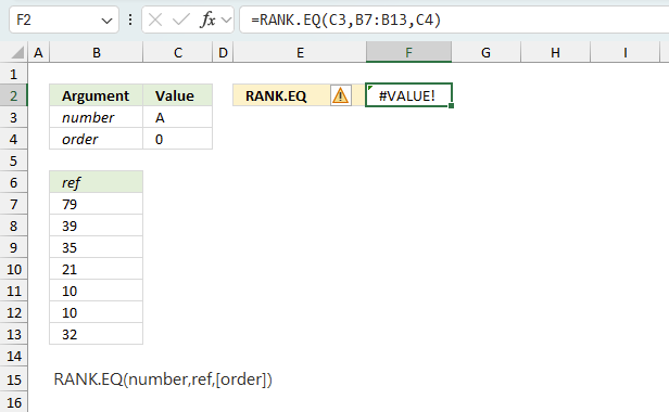
The RANK.EQ function returns
- #VALUE! error if you use a non-numeric input value.
- #NAME? error if you misspell the function name.
- propagates errors, meaning that if the input contains an error (e.g., #VALUE!, #REF!), the function will return the same error.
7.1 Troubleshooting the error value
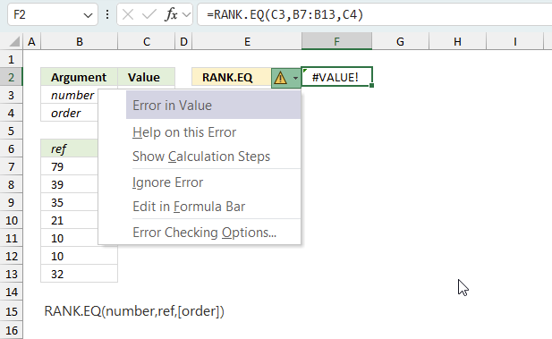
When you encounter an error value in a cell a warning symbol appears, displayed in the image above. Press with mouse on it to see a pop-up menu that lets you get more information about the error.
- The first line describes the error if you press with left mouse button on it.
- The second line opens a pane that explains the error in greater detail.
- The third line takes you to the "Evaluate Formula" tool, a dialog box appears allowing you to examine the formula in greater detail.
- This line lets you ignore the error value meaning the warning icon disappears, however, the error is still in the cell.
- The fifth line lets you edit the formula in the Formula bar.
- The sixth line opens the Excel settings so you can adjust the Error Checking Options.
Here are a few of the most common Excel errors you may encounter.
#NULL error - This error occurs most often if you by mistake use a space character in a formula where it shouldn't be. Excel interprets a space character as an intersection operator. If the ranges don't intersect an #NULL error is returned. The #NULL! error occurs when a formula attempts to calculate the intersection of two ranges that do not actually intersect. This can happen when the wrong range operator is used in the formula, or when the intersection operator (represented by a space character) is used between two ranges that do not overlap. To fix this error double check that the ranges referenced in the formula that use the intersection operator actually have cells in common.
#SPILL error - The #SPILL! error occurs only in version Excel 365 and is caused by a dynamic array being to large, meaning there are cells below and/or to the right that are not empty. This prevents the dynamic array formula expanding into new empty cells.
#DIV/0 error - This error happens if you try to divide a number by 0 (zero) or a value that equates to zero which is not possible mathematically.
#VALUE error - The #VALUE error occurs when a formula has a value that is of the wrong data type. Such as text where a number is expected or when dates are evaluated as text.
#REF error - The #REF error happens when a cell reference is invalid. This can happen if a cell is deleted that is referenced by a formula.
#NAME error - The #NAME error happens if you misspelled a function or a named range.
#NUM error - The #NUM error shows up when you try to use invalid numeric values in formulas, like square root of a negative number.
#N/A error - The #N/A error happens when a value is not available for a formula or found in a given cell range, for example in the VLOOKUP or MATCH functions.
#GETTING_DATA error - The #GETTING_DATA error shows while external sources are loading, this can indicate a delay in fetching the data or that the external source is unavailable right now.
7.2 The formula returns an unexpected value
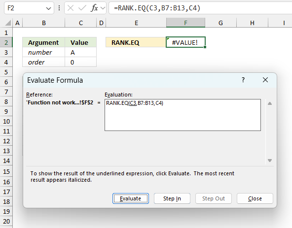
To understand why a formula returns an unexpected value we need to examine the calculations steps in detail. Luckily, Excel has a tool that is really handy in these situations. Here is how to troubleshoot a formula:
- Select the cell containing the formula you want to examine in detail.
- Go to tab “Formulas” on the ribbon.
- Press with left mouse button on "Evaluate Formula" button. A dialog box appears.
The formula appears in a white field inside the dialog box. Underlined expressions are calculations being processed in the next step. The italicized expression is the most recent result. The buttons at the bottom of the dialog box allows you to evaluate the formula in smaller calculations which you control. - Press with left mouse button on the "Evaluate" button located at the bottom of the dialog box to process the underlined expression.
- Repeat pressing the "Evaluate" button until you have seen all calculations step by step. This allows you to examine the formula in greater detail and hopefully find the culprit.
- Press "Close" button to dismiss the dialog box.
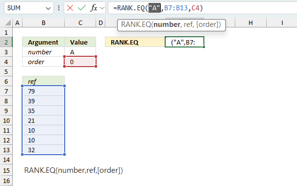
There is also another way to debug formulas using the function key F9. F9 is especially useful if you have a feeling that a specific part of the formula is the issue, this makes it faster than the "Evaluate Formula" tool since you don't need to go through all calculations to find the issue.
- Enter Edit mode: Double-press with left mouse button on the cell or press F2 to enter Edit mode for the formula.
- Select part of the formula: Highlight the specific part of the formula you want to evaluate. You can select and evaluate any part of the formula that could work as a standalone formula.
- Press F9: This will calculate and display the result of just that selected portion.
- Evaluate step-by-step: You can select and evaluate different parts of the formula to see intermediate results.
- Check for errors: This allows you to pinpoint which part of a complex formula may be causing an error.
The image above shows cell reference C3 converted to hard-coded value using the F9 key. The RANK.EQ function requires numerical values which is not the case in this example. We have found what is wrong with the formula.
Tips!
- View actual values: Selecting a cell reference and pressing F9 will show the actual values in those cells.
- Exit safely: Press Esc to exit Edit mode without changing the formula. Don't press Enter, as that would replace the formula part with the calculated value.
- Full recalculation: Pressing F9 outside of Edit mode will recalculate all formulas in the workbook.
Remember to be careful not to accidentally overwrite parts of your formula when using F9. Always exit with Esc rather than Enter to preserve the original formula. However, if you make a mistake overwriting the formula it is not the end of the world. You can “undo” the action by pressing keyboard shortcut keys CTRL + z or pressing the “Undo” button
7.3 Other errors
Floating-point arithmetic may give inaccurate results in Excel - Article
Floating-point errors are usually very small, often beyond the 15th decimal place, and in most cases don't affect calculations significantly.
Functions in 'Statistical' category
The RANK.EQ function function is one of 73 functions in the 'Statistical' category.
How to comment
How to add a formula to your comment
<code>Insert your formula here.</code>
Convert less than and larger than signs
Use html character entities instead of less than and larger than signs.
< becomes < and > becomes >
How to add VBA code to your comment
[vb 1="vbnet" language=","]
Put your VBA code here.
[/vb]
How to add a picture to your comment:
Upload picture to postimage.org or imgur
Paste image link to your comment.
Contact Oscar
You can contact me through this contact form