Extract unique distinct values sorted from A to Z
Table of Contents
- List a unique distinct list from a column sorted A to Z
- Extract a unique distinct list sorted from A-Z from range
1. List a unique distinct list from a column sorted A to Z
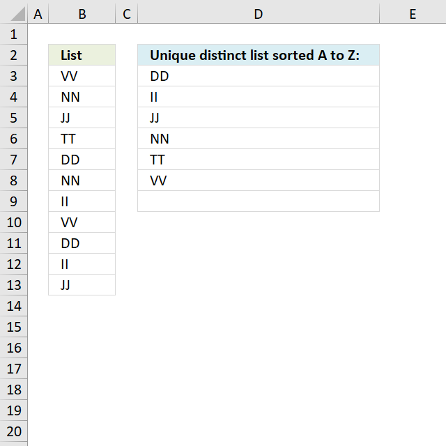
How do I create a unique distinct list from a column sorted A to Z using array formula?
Array formula in D3:
1.1 How to create an array formula
- Select cell D3.
- Copy (Ctrl + c) and paste (Ctrl + v) array formula into formula bar.
- Press and hold Ctrl + Shift.
- Press Enter once.
- Release all keys.

1.2 How to copy this array formula
- Select cell D3.
- Copy (Ctrl + C) cell D2.
- Select D3:D8
- Paste (CTRL + V)
1.3 How this array formula works
Step 1 - Filter unique distinct values
=INDEX($B$3:$B$13, MATCH(MIN(IF(COUNTIF($D$2:D2, $B$3:$B$13)=0,COUNTIF($B$3:$B$13, "<"&$B$3:$B$13)+1,9.9999E+307)), COUNTIF($B$3:$B$13, "<"&$B$3:$B$13)+1, 0))
COUNTIF($D$1:D1, List)=0
becomes
COUNTIF("Unique distinct list sorted A to Z:", {"VV";"NN";"JJ";"TT";"DD";"NN";"II";"VV";"DD";"II";"JJ"})=0
becomes
({0;0;0;0;0;0;0;0;0;0;0})=0
and returns {TRUE;TRUE;TRUE;TRUE;TRUE;TRUE;TRUE;TRUE;TRUE;TRUE;TRUE}.
Step 2 - Remove duplicate values from array
=INDEX($B$3:$B$13, MATCH(MIN(IF(COUNTIF($D$1:D1, $B$3:$B$13)=0,COUNTIF($B$3:$B$13, "<"&$B$3:$B$13)+1,9,9999E+307)), COUNTIF($B$3:$B$13, "<"&$B$3:$B$13)+1, 0))
MIN(IF(COUNTIF($D$1:D1, $B$3:$B$13)=0,COUNTIF($B$3:$B$13, "<"&$B$3:$B$13)+1,9,9999E+307))
becomes
MIN(IF({TRUE;TRUE;TRUE;TRUE;TRUE;TRUE;TRUE;TRUE;TRUE;TRUE;TRUE},{10;7;5;9;1;7;3;10;1;3;5},9,9999E+307))
becomes
MIN({10;7;5;9;1;7;3;10;1;3;5})
and returns 1.
Step 3 - Match smallest value
=INDEX($B$3:$B$13, MATCH(MIN(IF(COUNTIF($D$1:D1, $B$3:$B$13)=0,COUNTIF($B$3:$B$13, "<"&$B$3:$B$13)+1,9,9999E+307)), COUNTIF($B$3:$B$13, "<"&$B$3:$B$13)+1, 0))
MATCH(MIN(IF(COUNTIF($D$1:D1, $B$3:$B$13)=0,COUNTIF($B$3:$B$13, "<"&$B$3:$B$13)+1,9,9999E+307)), COUNTIF($B$3:$B$13, "<"&$B$3:$B$13)+1, 0)
becomes
MATCH(1, {10;7;5;9;1;7;3;10;1;3;5}, 0)
and returns 5.
Step 4 - Return a value or reference of the cell at the intersection of a particular row and column
=INDEX($B$3:$B$13, MATCH(MIN(IF(COUNTIF($D$1:D1, $B$3:$B$13)=0,COUNTIF($B$3:$B$13, "<"&$B$3:$B$13)+1,9,9999E+307)), COUNTIF($B$3:$B$13, "<"&$B$3:$B$13)+1, 0))
becomes
=INDEX($B$3:$B$13, 5)
becomes
=INDEX({"VV";"NN";"JJ";"TT";"DD";"NN";"II";"VV";"DD";"II";"JJ"}, 5)
and returns DD in cell D2.
1.4 Get Excel *.xlsx file
Unique-distinct-list-from-a-column-sorted-A-to-Z-using-array-formula11.xlsx
Extract a unique distinct list from a column sorted from A-Z - Excel 365 (Link)
2. Extract a unique distinct list sorted from A-Z from range
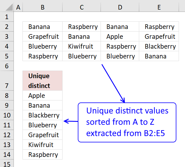
The image above shows an array formula in cell B8 that extracts unique distinct values sorted alphabetically from cell range B2:E5.
Array formula in B8:
Copy cell B8 and paste it to cells below as far as necessary.
To enter an array formula, type the formula in a cell then press and hold CTRL + SHIFT simultaneously, now press Enter once. Release all keys.
The formula bar now shows the formula with a beginning and ending curly bracket telling you that you entered the formula successfully. Don't enter the curly brackets yourself.
2.1 Explaining formula in cell B11
This formula consists of two parts, one extracts the row number and the other the column number needed to return the correct value.
INDEX(reference, row, col)
Step 1 to 6 shows how the row number is calculated, step 7 to 11 demonstrates how to calculate the column number.
Step 1 - Prevent duplicates
The COUNTIF function counts values based on a condition or criteria, in this case, we take into account previously displayed values in order to prevent duplicates in our output list.
COUNTIF($B$7:B7, $B$2:$E$5)=0
becomes
COUNTIF("Unique distinct", {"Banana", "Raspberry", "Banana", "Raspberry";"Grapefruit", "Banana", "Apple", "Grapefruit";"Blueberry", "Kiwifruit", "Raspberry", "Blackberry";"Raspberry", "Blueberry", "Blueberry", "Banana"})
becomes
{0,0,0,0;0,0,0,0;0,0,0,0;0,0,0,0}=0
and returns
{TRUE, TRUE, TRUE, TRUE;TRUE, TRUE, TRUE, TRUE;TRUE, TRUE, TRUE, TRUE;TRUE, TRUE, TRUE, TRUE}.
Step 2 - Replace TRUE with the corresponding rank order
The following IF function returns the corresponding sort order if the list had been sorted from A to Z based on the logical expression. FALSE returns "" (nothing).
IF(COUNTIF($B$7:B7,$B$2:$E$5)=0,COUNTIF($B$2:$E$5,"<"&$B$2:$E$5)+1,"")
becomes
IF({TRUE, TRUE, TRUE, TRUE;TRUE, TRUE, TRUE, TRUE;TRUE, TRUE, TRUE, TRUE;TRUE, TRUE, TRUE, TRUE}, {1,12,1,12;9,1,0,9;6,11,12,5;12,6,6,1}+1,"")
becomes
IF({TRUE, TRUE, TRUE, TRUE;TRUE, TRUE, TRUE, TRUE;TRUE, TRUE, TRUE, TRUE;TRUE, TRUE, TRUE, TRUE}, {1,12,1,12;9,1,0,9;6,11,12,5;12,6,6,1}+1,"")
becomes
IF({TRUE, TRUE, TRUE, TRUE;TRUE, TRUE, TRUE, TRUE;TRUE, TRUE, TRUE, TRUE;TRUE, TRUE, TRUE, TRUE}, {2,13,2,13;10,2,1,10;7,12,13,6;13,7,7,2},"")
and returns
{2,13,2,13;10,2,1,10;7,12,13,6;13,7,7,2}
Step 3 - Extract smallest value in array
The SMALL function extracts the k-th small number in array, in this case the second argument (k) is 1.
SMALL(IF(COUNTIF($B$7:B7, $B$2:$E$5)=0, COUNTIF($B$2:$E$5, "<"&$B$2:$E$5)+1, ""), 1)
becomes
SMALL({2,13,2,13;10,2,1,10;7,12,13,6;13,7,7,2}, 1)
and returns 1.
Step 4 - Replace TRUE with the corresponding row number
The IF function uses a logical expression to determine which value (argument) to return.
IF(SMALL(IF(COUNTIF($B$7:B7,$B$2:$E$5)=0,COUNTIF($B$2:$E$5,"<"&$B$2:$E$5)+1,""),1)=COUNTIF($B$2:$E$5,"<"&$B$2:$E$5)+1,ROW($B$2:$E$5)-MIN(ROW($B$2:$E$5))+1)
becomes
IF(1=COUNTIF($B$2:$E$5, "<"&$B$2:$E$5)+1, ROW($B$2:$E$5)-MIN(ROW($B$2:$E$5))+1)
becomes
IF(1={2,13,2,13;10,2,1,10;7,12,13,6;13,7,7,2}, ROW($B$2:$E$5)-MIN(ROW($B$2:$E$5))+1)
becomes
IF({FALSE,FALSE,FALSE,FALSE;FALSE,FALSE,TRUE,FALSE;FALSE,FALSE,FALSE,FALSE;FALSE,FALSE,FALSE,FALSE}, ROW($B$2:$E$5)-MIN(ROW($B$2:$E$5))+1)
becomes
IF({FALSE,FALSE,FALSE,FALSE;FALSE,FALSE,TRUE,FALSE;FALSE,FALSE,FALSE,FALSE;FALSE,FALSE,FALSE,FALSE}, {1;2;3;4})
and returns
{FALSE,FALSE,FALSE,FALSE;FALSE,FALSE,2,FALSE;FALSE,FALSE,FALSE,FALSE;FALSE,FALSE,FALSE,FALSE}
Step 5 - Find smallest value
The SMALL function finds the smallest value in the array ignoring the boolean values
SMALL(IF(SMALL(IF(COUNTIF($B$7:B7,$B$2:$E$5)=0,COUNTIF($B$2:$E$5,"<"&$B$2:$E$5)+1,""),1)=COUNTIF($B$2:$E$5,"<"&$B$2:$E$5)+1,ROW($B$2:$E$5)-MIN(ROW($B$2:$E$5))+1),1)
becomes
SMALL({FALSE,FALSE,FALSE,FALSE;FALSE,FALSE,2,FALSE;FALSE,FALSE,FALSE,FALSE;FALSE,FALSE,FALSE,FALSE},1)
and returns 2. This is the row number we need to extract the correct value from cell range B2:E5.
Step 6 - Return array
This step uses the INDEX function to return an array from a given row in cell range B2:E5.
INDEX(COUNTIF($B$2:$E$5, "<"&$B$2:$E$5)+1, SMALL(IF(SMALL(IF(COUNTIF($B$7:B7, $B$2:$E$5)=0, COUNTIF($B$2:$E$5, "<"&$B$2:$E$5)+1, ""), 1)=COUNTIF($B$2:$E$5, "<"&$B$2:$E$5)+1, ROW($B$2:$E$5)-MIN(ROW($B$2:$E$5))+1), 1), , 1)
becomes
INDEX(COUNTIF($B$2:$E$5, "<"&$B$2:$E$5)+1, 2, , 1)
becomes
INDEX({2,13,2,13;10,2,1,10;7,12,13,6;13,7,7,2}, 2, , 1)
and returns
{10,2,1,10}
Step 7 - Match value in array
This step uses the MATCH function to return the correct column number needed to extract the value we need from cell range B2:E5.
MATCH(MIN(IF(COUNTIF($B$7:B7, $B$2:$E$5)>0, "", COUNTIF($B$2:$E$5, "<"&$B$2:$E$5)+1)), INDEX(COUNTIF($B$2:$E$5, "<"&$B$2:$E$5)+1, SMALL(IF(SMALL(IF(COUNTIF($B$7:B7, $B$2:$E$5)=0, COUNTIF($B$2:$E$5, "<"&$B$2:$E$5)+1, ""), 1)=COUNTIF($B$2:$E$5, "<"&$B$2:$E$5)+1, ROW($B$2:$E$5)-MIN(ROW($B$2:$E$5))+1), 1), , 1), 0)
becomes
MATCH(MIN(IF(COUNTIF($B$7:B7, $B$2:$E$5)>0, "", COUNTIF($B$2:$E$5, "<"&$B$2:$E$5)+1)), {10,2,1,10}, 0)
becomes
MATCH(1, {10,2,1,10}, 0)
and returns 3. This is the column number we need.
Step 8 - Return value
INDEX($B$2:$E$5, SMALL(IF(SMALL(IF(COUNTIF($B$7:B7, $B$2:$E$5)=0, COUNTIF($B$2:$E$5, "<"&$B$2:$E$5)+1, ""), 1)=COUNTIF($B$2:$E$5, "<"&$B$2:$E$5)+1, ROW($B$2:$E$5)-MIN(ROW($B$2:$E$5))+1), 1), MATCH(MIN(IF(COUNTIF($B$7:B7, $B$2:$E$5)>0, "", COUNTIF($B$2:$E$5, "<"&$B$2:$E$5)+1)), INDEX(COUNTIF($B$2:$E$5, "<"&$B$2:$E$5)+1, SMALL(IF(SMALL(IF(COUNTIF($B$7:B7, $B$2:$E$5)=0, COUNTIF($B$2:$E$5, "<"&$B$2:$E$5)+1, ""), 1)=COUNTIF($B$2:$E$5, "<"&$B$2:$E$5)+1, ROW($B$2:$E$5)-MIN(ROW($B$2:$E$5))+1), 1), , 1), 0), 1)
becomes
=INDEX($B$2:$E$5, 3, 2)
and returns "Apple" in cell B8.
2.2 Get Excel *.xlsx file
Extract a unique distinct list sorted alphabetically from a range.xlsx
Extract unique distinct values A to Z from a range and ignore blanks - Excel 365
Unique distinct values category

First, let me explain the difference between unique values and unique distinct values, it is important you know the difference […]
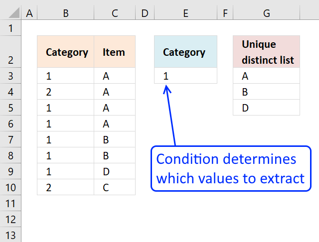
This article shows how to extract unique distinct values based on a condition applied to an adjacent column using formulas. […]
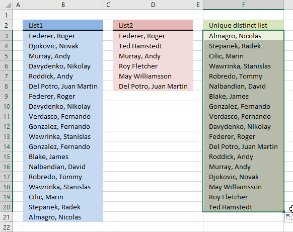
Question: I have two ranges or lists (List1 and List2) from where I would like to extract a unique distinct […]
Excel categories
10 Responses to “Extract unique distinct values sorted from A to Z”
Leave a Reply
How to comment
How to add a formula to your comment
<code>Insert your formula here.</code>
Convert less than and larger than signs
Use html character entities instead of less than and larger than signs.
< becomes < and > becomes >
How to add VBA code to your comment
[vb 1="vbnet" language=","]
Put your VBA code here.
[/vb]
How to add a picture to your comment:
Upload picture to postimage.org or imgur
Paste image link to your comment.
This is exactly what I've been looking for... almost. It breaks if there are blank cells in the named range. Is there a way to get this to work if there are blanks in the range?
Thanks.
Dave,
see this blog post: https://www.get-digital-help.com/extract-a-unique-distinct-list-sorted-alphabetically-removing-blanks-from-a-range-in-excel/
Hi Oscar!
Can you help me?
I have a name products column and their prices (other column).
I want to create unique distinct list with products name sorted by SUM of prices. Is it real using array formula?
Bill,
read this post:
Filter unique distinct list sorted based on sum of adjacent values
Thanks, Oscar!
I am using the following formula. How can i get it to work if there are blank cells?
How can i get it to work if there are formulas in the column?
=IFERROR(INDEX(List1,MATCH(MIN(IF(COUNTIF($F$9:F9,List1)=0,1,MAX((COUNTIF(List1,"<"&List1)+1)*2))*(COUNTIF(List1,"<"&List1)+1)),COUNTIF(List1,"<"&List1)+1,0)),"")
Jimmie,
try this formula:
=INDEX(List, MATCH(MIN(IF((List="")+COUNTIF(B1:$B$1, List), "", IF(ISNUMBER(List), COUNTIF(List, "<"&List), COUNTIF(List, "<"&List)+SUM(IF(ISNUMBER($A$2:$A$15), 1, 0))+1))), IF((List="")+COUNTIF(B1:$B$1, List), "", IF(ISNUMBER(List), COUNTIF(List, "<"&List), COUNTIF(List, "<"&List)+SUM(IF(ISNUMBER(List), 1, 0))+1)), 0)) Get the Excel file Unique-and-Sort-numbers-and-text-cells-using-excel-array-formula-works-with-formulas.xls
Oscar,
I need to sort from largest value to smallest and continue to have issues. I'm working with values and have flipped SMALL to LARGE and Min to MAX. I must be missing something simple, could you please point me in the correct direction?.
Appreciate all the help.
Alex
How about "Z to A"?
Thanks lots!
Thank You!