How to use the XLOOKUP function

This article demonstrates how to use the XLOOKUP function in Excel 365.
Table of Contents
- Example
- Syntax
- Arguments
- Video
- How to return multiple values
- How to search horizontally
- How to perform a reverse search - starting with the last item
- How to perform a binary xlookup
- How to perform a wildcard xlookup
- Get Excel *.xlsx file
- Search values distributed horizontally and return corresponding values
- Filter values distributed horizontally - Excel 365
- Function not working
1. Example

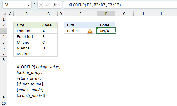
The XLOOKUP function lets you search one column for a search value, and return a corresponding value in another column from the same row.
Formula in cell F2:
The image above demonstrates the XLOOKUP function in cell F2, it uses a search value specified in cell E3 and searches column B.
A match is found in cell B5 and the corresponding value from column C is returned in cell F3.
2. Syntax

XLOOKUP(lookup_value, lookup_array, return_array, [if_not_found], [match_mode], [search_mode])
3. Arguments
| lookup_value | Required. The value you want to look up. |
| lookup_array | Required. This is a cell range or an array that you want to search. |
| return_array | Required. This is a cell range or an array that you want to return a result from. |
| [if_not_found] | Optional. A given text string is returned if a valid match is not found. #N/A is returned if this argument is omitted and a valid match is not found. |
| [match_mode] | Optional. Match setting:
0 - Exact match. Return #N/A if no valid match is found. (Default) -1 - Exact match. Return the next smaller item if no valid match is found. 1 - Exact match. Return the next larger item if no valid match is found. 2 - Wildcard match * - Any number of characters. Example, *son matches both "Johnson" and "Wilson" but not "Jones". ? - Any single character. Example, ?n matches both "in" and "on" but not "off". ~ (tilde) followed by ?, *, or ~ - Example, How~? matches How?. |
| [search_mode] | Optional. Search setting:
1 - Search starting at the first item. (Default) -1 - Reverse search starting at the last item. 2 - Binary search, lookup_array must be sorted in ascending order. -2 - Binary search, lookup_array must be sorted in descending order. |
4. Video
5. How to return multiple values

The formula below demonstrates the XLOOKUP function returning more values from the same row.
Formula in cell C6:
The return_array (3rd argument) contains two columns in this example. The lookup value is found in cell B8 and the corresponding values are in cell range C8:D8.
Note, the XLOOKUP function does not return multiple matches. It only returns the first valid match even if there are more valid matches.
I recommend that you use the FILTER function if you need to search for multiple values and return multiple corresponding values.
6. How to search horizontally

This example demonstrates how to lookup a value horizontally using the XLOOKUP function and return the corresponding value from the same column.
Search value "Milano" is found in cell E2 and the formula returns value "C" from row three in the same column.
Formula in cell C6:
7. How to find the last match - reverse search

The image above shows the XLOOKUP function in cell C3, it searches cell range B6:B12 starting at the last value.
There are two matches cells B8 and B11, however, the search starts at the last value and the first matching value is in cell B11. The corresponding value is in cell C11.
Formula in cell C3:
The last argument lets you choose the search mode.
XLOOKUP(lookup_value, lookup_array, return_array, [if_not_found], [match_mode], [search_mode])
-1 : Reverse search starting at the last item.
This article explains how to do it in earlier Excel versions: Find last matching value in an unsorted table
8. How to do a binary XLOOKUP

This example demonstrates how to do a binary lookup using the XLOOKUP function.
Make sure the lookup_array is sorted appropriately based on the chosen value in the last argument.
Formula in cell C3:
The last argument lets you choose the search mode.
XLOOKUP(lookup_value, lookup_array, return_array, [if_not_found], [match_mode], [search_mode])
2 : Binary search, lookup_array must be sorted in ascending order.
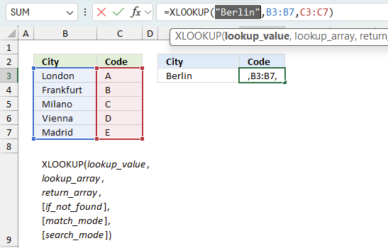
9. How to do a wildcard XLOOKUP

The image above demonstrates how to do a wildcard lookup using the XLOOKUP function.
The asterisk matches any number of characters. M* matches both Milano and Madrid, however, Milano is the first match in the list. The corresponding value is "C" and that is returned in cell F3.
Formula in cell C3:
The second last argument lets you choose the match mode.
XLOOKUP(lookup_value, lookup_array, return_array, [if_not_found], [match_mode], [search_mode])
* - Any number of characters.
? - Any single character.
~ (tilde) followed by ?, *, or ~
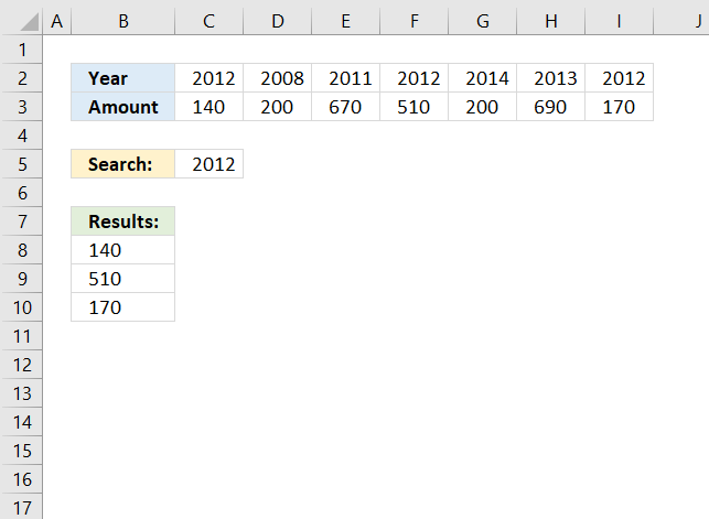
11. Search values distributed horizontally and return corresponding values
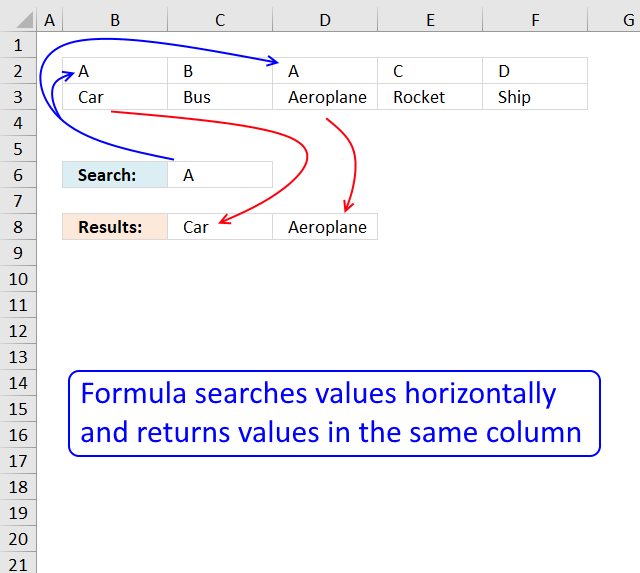
Question: Hi, The formula here works great but I can't figure out how to change it to work with data in columns.
Here is what I have:
=INDEX(A2:E2,SMALL(IF(A1:E1=A3,COLUMN(A1:E1),""),COLUMN()))
A B C D E
1 A B A C D
2 Car Bus Aeroplane Rocket Ship
3 A
I'd expect the result to read:
A B
4 Car Aeroplane
...but instead I get
A B
4 #NUM #NUM
Can you offer any advice?
This is a question from Using array formula to look up multiple values in a list
Answer:
Array formula in cell B8:
To enter an array formula, type the formula in a cell then press and hold CTRL + SHIFT simultaneously, now press Enter once. Release all keys.
The formula bar now shows the formula with a beginning and ending curly bracket telling you that you entered the formula successfully. Don't enter the curly brackets yourself.
Explaining formula in cell B8
Step 1 - Check if lookup value is equal to values in cell range C2:I2
The IF function has three arguments, the first one must be a logical expression. If the expression evaluates to TRUE then one thing happens (argument 2) and if FALSE another thing happens (argument 3). The following lines explain the logical expression:
$C$2:$I$2=$C$5
becomes
{2012,2008,2011,2012,2014,2013,2012}=2012
and returns
{TRUE,FALSE,FALSE,TRUE,FALSE,FALSE,TRUE}
Step 2 - Return corresponding column number
The column number will help us identify the values we want to return from another row. TRUE - corresponding column number, FALSE - nothing "".
IF($C$2:$I$2=$C$5, MATCH(COLUMN($C$2:$I$2), COLUMN($C$2:$I$2)), "")
becomes
IF({TRUE,FALSE,FALSE,TRUE,FALSE,FALSE,TRUE}, MATCH(COLUMN($C$2:$I$2), COLUMN($C$2:$I$2)), "")
becomes
IF({TRUE,FALSE,FALSE,TRUE,FALSE,FALSE,TRUE}, {1,2,3,4,5,6,7}, "")
and returns
{1,"","",4,"","",7}.
Step 3 - Extract k-th smallest column number
To be able to return a new value in a cell each I use the SMALL function to filter column numbers from smallest to largest.
The ROWS function keeps track of the numbers based on an expanding cell reference. It will expand as the formula is copied to the cells below.
SMALL(IF($C$2:$I$2=$C$5, MATCH(COLUMN($C$2:$I$2), COLUMN($C$2:$I$2)), ""), ROWS($A$1:A1))
becomes
SMALL({1,"","",4,"","",7}, ROWS($A$1:A1))
becomes
SMALL({1,"","",4,"","",7}, 1)
and returns 1.
Step 4 - Return value based on column number
The INDEX function returns a value based on a cell reference and column/row numbers.
INDEX($C$3:$I$3, SMALL(IF($C$2:$I$2=$C$5, MATCH(COLUMN($C$2:$I$2), COLUMN($C$2:$I$2)), ""), ROWS($A$1:A1)))
becomes
INDEX($C$3:$I$3, 1)
becomes
INDEX({140,200,670,510,200,690,170}, 1)
and returns 140 in cell B8.
12. Filter values distributed horizontally - Excel 365

The FILTER function is capable to filter values arranged horizontally as well, the TRANSPOSE function rearranges the result vertically.
Excel 365 formula in cell B8:
Explaining formula
Step 1 - Logical test
The equal sign is a logical operator, it allows you to compare value to value. The result is a boolean value TRUE or FALSE.
C2:I2=C5
becomes
{2012,2008,2011,2012,2014,2013,2012}=2012
and returns
{TRUE, FALSE, FALSE, TRUE, FALSE, FALSE, TRUE}.
Step 2 - Filter values
The FILTER function extracts values/rows based on a condition or criteria.
Function syntax: FILTER(array, include, [if_empty])
FILTER(C3:I3,C2:I2=C5)
becomes
FILTER({140, 200, 670, 510, 200, 690, 170},{TRUE, FALSE, FALSE, TRUE, FALSE, FALSE, TRUE})
and returns
{140, 510, 170}.
Step 3 - Transpose values
The TRANSPOSE function converts a vertical range to a horizontal range, or vice versa.
Function syntax: TRANSPOSE(array)
TRANSPOSE(FILTER(C3:I3,C2:I2=C5))
becomes
TRANSPOSE({140, 510, 170})
and returns
{140; 510; 170}.
13. Function not working
The XLOOKUP function returns
- #N/A error if you use a lookup_value that does not exist in the lookup_array.
- #NAME? error if you misspell the function name.
- propagates errors, meaning that if the input contains an error (e.g., #VALUE!, #REF!), the function will return the same error.
13.1 Troubleshooting the error value
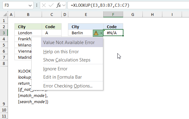
When you encounter an error value in a cell a warning symbol appears, displayed in the image above. Press with mouse on it to see a pop-up menu that lets you get more information about the error.
- The first line describes the error if you press with left mouse button on it.
- The second line opens a pane that explains the error in greater detail.
- The third line takes you to the "Evaluate Formula" tool, a dialog box appears allowing you to examine the formula in greater detail.
- This line lets you ignore the error value meaning the warning icon disappears, however, the error is still in the cell.
- The fifth line lets you edit the formula in the Formula bar.
- The sixth line opens the Excel settings so you can adjust the Error Checking Options.
Here are a few of the most common Excel errors you may encounter.
#NULL error - This error occurs most often if you by mistake use a space character in a formula where it shouldn't be. Excel interprets a space character as an intersection operator. If the ranges don't intersect an #NULL error is returned. The #NULL! error occurs when a formula attempts to calculate the intersection of two ranges that do not actually intersect. This can happen when the wrong range operator is used in the formula, or when the intersection operator (represented by a space character) is used between two ranges that do not overlap. To fix this error double check that the ranges referenced in the formula that use the intersection operator actually have cells in common.
#SPILL error - The #SPILL! error occurs only in version Excel 365 and is caused by a dynamic array being to large, meaning there are cells below and/or to the right that are not empty. This prevents the dynamic array formula expanding into new empty cells.
#DIV/0 error - This error happens if you try to divide a number by 0 (zero) or a value that equates to zero which is not possible mathematically.
#VALUE error - The #VALUE error occurs when a formula has a value that is of the wrong data type. Such as text where a number is expected or when dates are evaluated as text.
#REF error - The #REF error happens when a cell reference is invalid. This can happen if a cell is deleted that is referenced by a formula.
#NAME error - The #NAME error happens if you misspelled a function or a named range.
#NUM error - The #NUM error shows up when you try to use invalid numeric values in formulas, like square root of a negative number.
#N/A error - The #N/A error happens when a value is not available for a formula or found in a given cell range, for example in the VLOOKUP or MATCH functions.
#GETTING_DATA error - The #GETTING_DATA error shows while external sources are loading, this can indicate a delay in fetching the data or that the external source is unavailable right now.
13.2 The formula returns an unexpected value
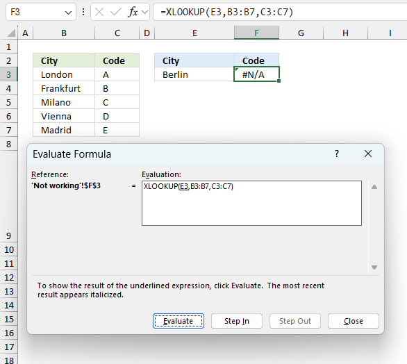
To understand why a formula returns an unexpected value we need to examine the calculations steps in detail. Luckily, Excel has a tool that is really handy in these situations. Here is how to troubleshoot a formula:
- Select the cell containing the formula you want to examine in detail.
- Go to tab “Formulas” on the ribbon.
- Press with left mouse button on "Evaluate Formula" button. A dialog box appears.
The formula appears in a white field inside the dialog box. Underlined expressions are calculations being processed in the next step. The italicized expression is the most recent result. The buttons at the bottom of the dialog box allows you to evaluate the formula in smaller calculations which you control. - Press with left mouse button on the "Evaluate" button located at the bottom of the dialog box to process the underlined expression.
- Repeat pressing the "Evaluate" button until you have seen all calculations step by step. This allows you to examine the formula in greater detail and hopefully find the culprit.
- Press "Close" button to dismiss the dialog box.
There is also another way to debug formulas using the function key F9. F9 is especially useful if you have a feeling that a specific part of the formula is the issue, this makes it faster than the "Evaluate Formula" tool since you don't need to go through all calculations to find the issue..
- Enter Edit mode: Double-press with left mouse button on the cell or press F2 to enter Edit mode for the formula.
- Select part of the formula: Highlight the specific part of the formula you want to evaluate. You can select and evaluate any part of the formula that could work as a standalone formula.
- Press F9: This will calculate and display the result of just that selected portion.
- Evaluate step-by-step: You can select and evaluate different parts of the formula to see intermediate results.
- Check for errors: This allows you to pinpoint which part of a complex formula may be causing an error.
The image above shows cell reference E3 converted to hard-coded value using the F9 key. The XLOOKUP function requires a valid lookup_value that exists in the lookup_array, which is not the case in this example. We have found what is wrong with the formula.
Tips!
- View actual values: Selecting a cell reference and pressing F9 will show the actual values in those cells.
- Exit safely: Press Esc to exit Edit mode without changing the formula. Don't press Enter, as that would replace the formula part with the calculated value.
- Full recalculation: Pressing F9 outside of Edit mode will recalculate all formulas in the workbook.
Remember to be careful not to accidentally overwrite parts of your formula when using F9. Always exit with Esc rather than Enter to preserve the original formula. However, if you make a mistake overwriting the formula it is not the end of the world. You can “undo” the action by pressing keyboard shortcut keys CTRL + z or pressing the “Undo” button
13.3 Other errors
Floating-point arithmetic may give inaccurate results in Excel - Article
Floating-point errors are usually very small, often beyond the 15th decimal place, and in most cases don't affect calculations significantly.
Useful links
XLOOKUP function - Microsoft
How To Use the XLOOKUP Function in Excel
'XLOOKUP' function examples
I will in this article demonstrate how to use the VLOOKUP function with multiple conditions. The function was not built […]
Functions in 'Lookup and reference' category
The XLOOKUP function function is one of 25 functions in the 'Lookup and reference' category.
Excel function categories
Excel categories
10 Responses to “How to use the XLOOKUP function”
Leave a Reply
How to comment
How to add a formula to your comment
<code>Insert your formula here.</code>
Convert less than and larger than signs
Use html character entities instead of less than and larger than signs.
< becomes < and > becomes >
How to add VBA code to your comment
[vb 1="vbnet" language=","]
Put your VBA code here.
[/vb]
How to add a picture to your comment:
Upload picture to postimage.org or imgur
Paste image link to your comment.
That works fantastically! Thanks very much. A great way to start on a Monday morning!
i have two colums
department NO
sales 2
computers 1
laptops 1
books 2
i am doing lookup but
getting result is
2 books - i should get "sales" here
2 books
1 laptops - i should get "computers" here
1 laptops
Could you please help me out
rave,
Read this post: How to return multiple values using vlookup
=INDEX($A$2:$E$2, SMALL(IF($A$1:$E$1=$A$3, COLUMN($A$1:$E$1)-MIN(COLUMN($A$1:$E$1))+1, ""), COLUMNS($A:A)) + CTRL + SHIFT + ENTER
Works great, however if the criteria is not in the table, I need the cell to be blank. E.g ISNA for a vlookup etc excel2003.
Thanks
Ross,
=IFERROR(INDEX($A$2:$E$2, SMALL(IF($A$1:$E$1=$A$3, COLUMN($A$1:$E$1)-MIN(COLUMN($A$1:$E$1))+1, ""), COLUMNS($A:A)), "")
I'm having trouble with a formula. I need it to look at another sheet within the same workbook, and pull information. My sheet looks like this:
Last Name First Name Grade TCH Status Required Class CH
Thomas John 7 New 12 PHN01 10
It goes on to list 7 more Class and CH columns. Teachers have signed up for classes and I have a spreadsheet with their choices. I want to make sign in sheets but have excel automatically pull the teachers first and last name from the sheet they signed up on. I'm hoping this can be done automatically...:)
Nancy,
Can you explain in greater detail?
I want to make sign in sheets but have excel automatically pull the teachers first and last name from the sheet they signed up on
Do you want multiple drop down list containing all the teachers last and first names?
I have a table of dates C32:I82. Each column represents a different type of day off. However, all dates in the range are included in total days off. I want to extract all dates from the range that fall between a start and an end date and store it in another range. I am having great difficulty with this as I am a novice at best.
Wil R.
However, all dates in the range are included in total days off
Can you explain in greater detail?
i have below table
name 12/1/2020|13/1/2020|14/1/2020|Firs date| second date| third Date
A 1 | | 1 | | |
B | 1 | 1 | | |
and i want formula to get Firs date, second date and third date if its available.