Partial match for multiple strings – AND logic

This article demonstrates formulas that let you perform partial matches based on multiple strings and return those strings if all match the same cell. This is AND logic meaning all conditions must be met.
Table of contents
- Partial match for multiple strings - AND logic - returns the first match
- Partial match for multiple strings - AND logic - returns all matches
- Partial match for multiple strings - AND logic - returns all matches (Excel 365)
- Partial match for multiple strings - AND logic - returns all corresponding values
- Get Excel file
- Return multiple matches with wildcard VLOOKUP
1. Partial match for multiple strings - AND logic - returns the first match
This regular formula returns the first cell that contains both strings from cell range B3:B13, this is not a case-sensitive match.
Formula in cell E6:
1.1 Explaining formula
Step 1 - Partial match based on the first condition
The SEARCH function returns a number representing the position of character at which a specific text string is found reading left to right. It is not a case-sensitive search.
SEARCH($E$2, $B$3:$B$13)
returns {#VALUE!; 1; 2; ...; 3}.
Notice the error values, this happens when the SEARCH function can't find the string.
Step 2 - Partial match based on second condition
SEARCH($E$3, $B$3:$B$13)
returns {1; #VALUE!; ...; 1}.
Step 3 - Multiply arrays AND logic
We need to find cells that contain both strings, we can identify those cells by multiplying the arrays. The result will be a number if both strings are found in the same cell.
Here is the logic behind the calculation:
#VALUE! * number = #VALUE!
number * #VALUE! = #VALUE!
number * number = number
SEARCH($E$2, $B$3:$B$13)*SEARCH($E$3, $B$3:$B$13)
returns {#VALUE!; #VALUE!; ... ; 3}.
Step 4 - Identify numbers
The ISNUMBER function returns TRUE if value is a number and FALSE if not, this works also with error values meaning #VALUE! returns FALSE.
ISNUMBER(value)
ISNUMBER(SEARCH($E$2, $B$3:$B$13)*SEARCH($E$3, $B$3:$B$13))
returns {FALSE; FALSE; ... ; TRUE}.
Step 5 - Find position of first TRUE in array
The MATCH function returns the relative position of an item in an array or cell reference that matches a specified value in a specific order.
MATCH(lookup_value, lookup_array, [match_type])
MATCH(TRUE, ISNUMBER(SEARCH($E$2, $B$3:$B$13)*SEARCH($E$3, $B$3:$B$13)), 0)
returns 8.
Step 6 - Return value from cell range B3:B13
The INDEX function returns a value from a cell range, you specify which value based on a row and column number.
INDEX($B$3:$B$13, MATCH(TRUE, ISNUMBER(SEARCH($E$2, $B$3:$B$13)*SEARCH($E$3, $B$3:$B$13)), 0))
returns "BFA".
2. Partial match for multiple strings - AND logic - returns all values

This regular formula returns the all cell values that contain both strings from cell range B3:B13, this is not a case-sensitive match.
Formula in cell E6:
1.1 Explaining formula
Step 1 - Partial match based on the first condition
The SEARCH function returns a number representing the position of character at which a specific text string is found reading left to right. It is not a case-sensitive search.
SEARCH($E$2, $B$3:$B$13)
returns {#VALUE!; 1; .. ; 3}.
Notice the error values, they appear if the string is not found at all.
Step 2 - Partial match based on the second condition
SEARCH($E$3, $B$3:$B$13)
returns {1; #VALUE!;... ; 1}.
Step 3 - Multiply arrays
We need to find cells that contain both strings, we can identify those cells by multiplying the arrays. The result will be a number if both strings are found in the same cell.
Here is the logic behind the calculation:
#VALUE! * number = #VALUE!
number * #VALUE! = #VALUE!
number * number = number
SEARCH($E$2, $B$3:$B$13)*SEARCH($E$3, $B$3:$B$13)
returns {#VALUE!; #VALUE!; ... ; 3}.
Step 4 - Identify numbers
The ISNUMBER function returns TRUE if value is a number and FALSE if not, this works also with error values meaning #VALUE! returns FALSE.
ISNUMBER(value)
ISNUMBER(SEARCH($E$2, $B$3:$B$13)*SEARCH($E$3, $B$3:$B$13))
returns {FALSE; FALSE; ... ; TRUE}.
Step 5 - Replace True with row number
The IF function returns one value if the logical test is TRUE and another value if the logical test is FALSE.
IF(logical_test, [value_if_true], [value_if_false])
We want to substitute True with the corresponding row number in order to get the correct value in step 7.
The ROW function calculates the row number of a cell reference.
ROW(reference)
This works fine with a reference to a cell range as well, the function returns an array of numbers.
ROW($B$3:$B$13) returns {3; 4; ... ; 13}
The MATCH function returns the relative position of an item in an array or cell reference that matches a specified value in a specific order.
MATCH(lookup_value, lookup_array, [match_type])
MATCH(ROW($B$3:$B$13), ROW($B$3:$B$13))
returns {1; 2; ... ; 11}.
IF(ISNUMBER(SEARCH($E$2, $B$3:$B$13)*SEARCH($E$3, $B$3:$B$13)), MATCH(ROW($B$3:$B$13), ROW($B$3:$B$13)))
returns {FALSE; FALSE; ... ; 11}.
Step 6 - Get the k-th smallest row number
The SMALL function returns the k-th smallest value from a group of numbers. The first argument is a cell range or array that you want to find the k-th smallest number from. The SMALL function ignores text and boolean values.
SMALL(array, k)
SMALL(IF(ISNUMBER(SEARCH($E$2, $B$3:$B$13)*SEARCH($E$3, $B$3:$B$13)), MATCH(ROW($B$3:$B$13), ROW($B$3:$B$13))), ROWS($A$1:A1))
The ROWS function returns a number representing the number of rows in a reference.
ROWS(ref)
ROWS($A$1:A1) contains the following cell reference $A$1:A1, it contains both an absolute and relative cell reference making it a growing cell reference. This means that when the formula is copied to cells below the cell reference expands automatically. This will return a larger number for each cell below making the formula get a new row number in each cell.
SMALL({FALSE; FALSE; ... ; 11}, ROWS($A$1:A1))
returns 4.
Step 7 - Get value
The INDEX function returns a value from a cell range, you specify which value based on a row and column number.
INDEX($B$3:$B$13, SMALL(IF(ISNUMBER(SEARCH($E$2, $B$3:$B$13)*SEARCH($E$3, $B$3:$B$13)), MATCH(ROW($B$3:$B$13), ROW($B$3:$B$13))), ROWS($A$1:A1)))
returns the value in cell B6 which is "ABF". The fourth cell in $B$3:$B$13 is cell B6.
3. Partial match for multiple strings - AND logic - returns all matches (Excel 365)

The following formula extracts values from cell range B3:B13 if both strings are found in a cell, in other words, a partial match for both conditions.
Notice that the formula is much smaller than the previous Excel versions. The new FILTER function is great, it simplifies the formula and makes it easier to understand.
Dynamic array formula in cell E6:
Explaining formula in cell E6
Step 1 - Partial match based on the first condition
The SEARCH function returns a number representing the position of character at which a specific text string is found reading left to right. It is not a case-sensitive search.
SEARCH($E$2, $B$3:$B$13)
returns {#VALUE!; 1; ... ; 3}.
Notice the error values, they appear if the string is not found at all.
Step 2 - Partial match based on the second condition
SEARCH($E$3, $B$3:$B$13)
returns {1; #VALUE!; ... ; 1}.
Step 3 - Multiply arrays
We need to find cells that contain both strings, we can identify those cells by multiplying the arrays. The result will be a number if both strings are found in the same cell.
Here is the logic behind the calculation:
#VALUE! * number = #VALUE!
number * #VALUE! = #VALUE!
number * number = number
SEARCH($E$2, $B$3:$B$13)*SEARCH($E$3, $B$3:$B$13)
returns {#VALUE!; #VALUE!; ... ; 3}.
Step 4 - Identify numbers
The ISNUMBER function returns TRUE if value is a number and FALSE if not, this works also with error values meaning #VALUE! returns FALSE.
ISNUMBER(value)
ISNUMBER(SEARCH($E$2, $B$3:$B$13)*SEARCH($E$3, $B$3:$B$13))
returns {FALSE; FALSE; ... ; TRUE}.
Step 5 - Get values
The FILTER function lets you extract values/rows based on a condition or criteria. It is in the Lookup and reference category and is only available to Excel 365 subscribers.
FILTER(B3:B13, ISNUMBER(SEARCH($E$2, $B$3:$B$13)*SEARCH($E$3, $B$3:$B$13)))
returns {"BFA"; "FDB"}.
4. Partial match for multiple strings - AND logic - returns all corresponding values

This formula extracts values from cell range C3:C13 if the corresponding cell in B3;B13 contains both strings specified in cell F2 and F3.
The formula is almost identical to the formula in section 2, only the first cell reference is changed.
Array formula in cell F6:
Read the explanation in section 2 if you want to know more about the formula.
5. Get Excel file
6. Return multiple matches with wildcard VLOOKUP

Mr.Excel had a "challenge of the month" June/July 2008 about Wildcard VLOOKUP:
"The data in column A contains a series of phrases. Every phrase contains one color in the phrase. The goal of the challenge is to use the lookup table in D2:E10 to assign the phrase to one of the names in column E."
Source: https://www.mrexcel.com/pc18.shtml
The winner created this formula to return last match in the range:
The third winner used circular reference and iterations to return multiple matches.
How to return multiple matches without circular references

Excel 365 formula in cell C2:
Array formula in cell C2:
Recommended article:
Recommended articles
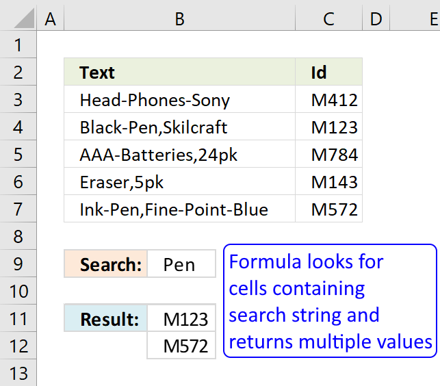
This article demonstrates array formulas that search for cell values containing a search string and returns corresponding values on the […]
Alternative array formula in C2:
How to create an array formula
- Select cell C2
- Copy above array formula
- Paste to formula bar
- Press and hold Ctrl + Shift
- Press Enter once
- Release all keys
Copy cell C2 and paste it right as far as needed. Then copy cells and paste down as far as needed.
How to copy array formula
- Select cell C2
- Copy (Ctrl + c)
- Select cell D2
- Paste (Ctrl + v)
Explaining array formula in cell C2
Step 1 - Find text string
The COUNTIF function counts values based on a condition or criteria, in this case two asterisks are appended to the second argument. This makes the COUNTIF function count any value that contains the string, asterisk matches zero or more characters.
COUNTIF($A2,"*"&$F$2:$F$12&"*")
returns {1; 0; ... ; 0}
Step 2 - Convert array to row numbers
The IF function has three arguments, the first one must be a logical expression. If the expression evaluates to TRUE then one thing happens (argument 2) and if FALSE another thing happens (argument 3).
IF(COUNTIF($A2,"*"&$F$2:$F$12&"*"), ROW($F$1:$F$11), "")
returns {1; ""; "... ; 10; ""}
Step 3 - Return the k-th smallest row number in this data set
To be able to return a new value in a cell each I use the SMALL function to filter column numbers from smallest to largest. SMALL( array, k) The second argument changes when the cell is copied to cells below, this will extract a new value in each cell.
SMALL(IF(COUNTIF($A2,"*"&$F$2:$F$12&"*"), ROW($F$1:$F$11), ""), COLUMN(A1))
becomes
SMALL({1; ""; ""; ""; ""; ""; ""; ""; ""; 10; ""},1)
and returns 1.
Step 4 - Return a value or reference of the cell at the intersection of a particular row and column
The INDEX function returns a value based on a cell reference and column/row numbers.
INDEX($G$2:$G$12, SMALL(IF(COUNTIF($A2,"*"&$F$2:$F$12&"*"), ROW($F$1:$F$11), ""), COLUMN(A1)))
returns "Joe" in cell C2.
Search and return multiple values category
This article demonstrates array formulas that search for cell values containing a search string and returns corresponding values on the […]
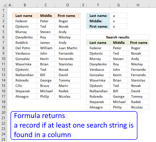
RU asks: Can you please suggest if i want to find out the rows with fixed value in "First Name" […]
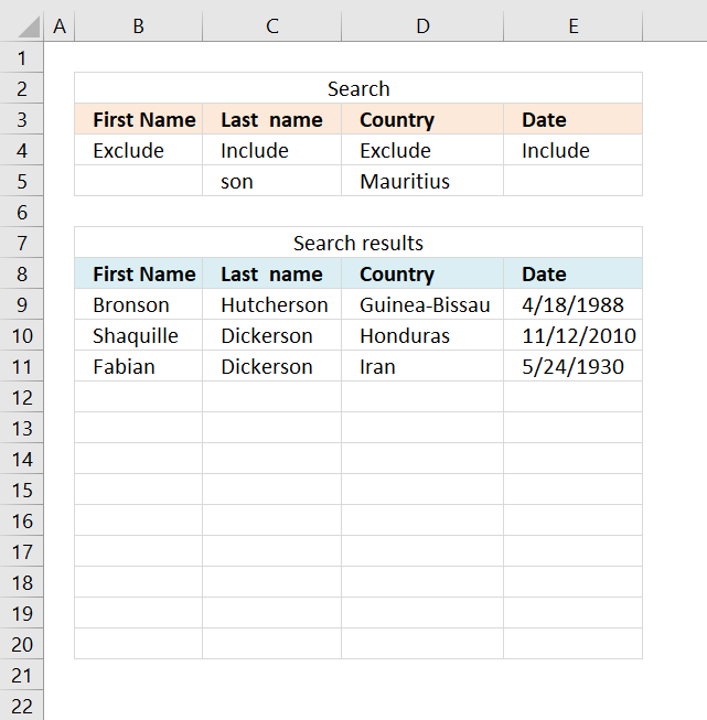
This article demonstrates three different ways to filter a data set if a value contains a specific string and if […]
Excel categories
29 Responses to “Partial match for multiple strings – AND logic”
Leave a Reply
How to comment
How to add a formula to your comment
<code>Insert your formula here.</code>
Convert less than and larger than signs
Use html character entities instead of less than and larger than signs.
< becomes < and > becomes >
How to add VBA code to your comment
[vb 1="vbnet" language=","]
Put your VBA code here.
[/vb]
How to add a picture to your comment:
Upload picture to postimage.org or imgur
Paste image link to your comment.
If the list of strings in column D was to increase to a large number e.g. 15, how would you tell excell to select the range of strings, so that you don't have to select each string "SEARCH($D$3" in the search parameter, as it seems is the case at the moment?
Interesting question! I will look into this as soon as possible. Thanks for commenting!
See this blog post: Search for multiple text strings in multiple cells in excel, part 2
Jerome, see this blog post: https://www.get-digital-help.com/search-and-display-all-cells-that-contain-all-search-strings-in-excel/
can you please modify the function (f2:f11) to display the text strings in CELL G.. disregard the ROW NUMBER Display thnx
the function will be in data validation.. and it will display 2 outputs in the list
PIPO,
I have now updated this blog post. The array formula is now easier to work with. Only copy the formula to your worksheet and create the named ranges.
Thanks for bringing this post to my attention.
Oscar,
Thank you sir, but if i put the array formula directly in the data validation list.. it only display "BFA" in the list.. i don't want to create a name range for the search result to display in data validation... thanks again in advance
PIPO,
I don´t know how to use an array formula in a data validation list. It seems to only "accept" a range of values.
Very interesting question, maybe someone else has an answer?
But I managed to create a "custom" data validation, see this post: https://www.get-digital-help.com/search-for-multiple-text-strings-in-multiple-cells-and-use-in-data-validation-in-excel/
Oscar,
Thanks you, it's a very helpful website. Would you able to search for those text strings (Search_Strings) contained in each cell then show? (cell contained both D2:D3 then show). Thanks,
James, can you explain in greater detail? I don´t understand.
Oscar, how can I use the Text_col on a different sheet in the same worksheet?
Text_col is a named range. Select a new range on a different sheet.
Oscar,
Rather than display the values could you collate them as part of a sum?
I have a a sheet that i could use a little help with, is thee any chance you could give me some advise?
Thanks
Daniel.
Daniel,
Array formula in cell E10:
Get the Excel file
search and sum.xls
I have used the winning solution for my cause and it helped me a lot and saved a lot of very valuable time!!!
THANK YOU VERY MUCH for your kind help.
Andrey
LOOKUP(2^15,SEARCH(D$2:D$10,A2),E$2:E$10)
Anyone explain this formula step by step..because i don't understand the function of the formula....
I totally agree with Ahmed.
I ma intrigued by the formula that won. I totally get the "lookup" and the "search" portions of it but I do NOT understand the "2^15". What function is this performing? How does this work? I can't even find anything online that resembles it (other than in its simplest form of "2 to the 15th power").
Can you offer some insight???
Hi,
My table array has wildcards that is of the format "ABCD****" or sometimes "ABCDE***" or sometimes "ABCDEF**". The main sheet contains that data of the format "ABCDEFGH" and needs to fetch an account from another cell in Sheet2(that contains the array).
Kindly help with handling this case.
Thanks,
CK.
CK,
Perhaps you are looking for this post:
Search for a text string and return multiple adjacent values
Oscar ,
Thank you, it's a very helpful website . I need your help in excel search . I have two Columns Cola with more than 10,000 records and Column B with 500 records. I need to show all the rows of Column A which contains case sensitive match of any records from column B.
is this possible? I have multiple terminal IDs and need to convert them into a location. This is just the beginning of the 'if' statement with 2 of the beginning ID numbers. I am using a table.
=IF(A25="@ ATM Deposit 0087*",VLOOKUP("@ ATM Deposit 0087*",$A4:$B18,2,FALSE),IF(A25="@ ATM Deposit 0487*",VLOOKUP("@ ATM Deposit 0487*",$A4:$B18,2,FALSE)))
Hopefully you can help me!! I'm using this formula with no issues: =+IF(C24="","",IFERROR(INDEX('Edited Data'!$P$2:$P$300,SMALL(IF(C24='Edited Data'!$N$2:$N$300,ROW('Edited Data'!$N$2:$N$300)-ROW('Edited Data'!$N$2)+1),COLUMN('Edited Data'!$A$1))),""))
Basically, C24 is a name, and it's looking for that name in N2:N300 on a tab called Edited Data. It works perfectly, but instead of looking for the name, I want it to look for the name as a wild card. 99% of the time it works, but sometimes the name is apart of a string of text and that formula doesn't pick it up. I'm OK with having it done manually if necessary, but if I can have it look for *C24* instead of C24, that would be amazing!!
I used the Alternative formula. When I copy down the formula, it's giving me error: #NUM!
Hi Oscar,
Tks for the "Return multiple matches with wildcard vlookup in excel" formula " =LOOKUP(2^15,SEARCH(D$2:D$10,A2),E$2:E$10)" whick worked 100% for me. Is it possible to get it to an exact match? eg If I use Brown as the keyword to lookup then it would find brown and brownish, etc?
Tks!
what if I had to print the adjacent column value, consider B is the named range(Text_col), but I want the value in column A, how should I tweak the code?
2 things.
1. Your explanation references COUNTIF, but the actual formula uses ISNUMBER(SEARCH(...)). I can only assume this is because COUNTIF doesn't appear to maintain array awareness the way it is depicted in the explanation.
2. I did find this useful in addressing a related problem I was having, so I thought I would share back. The following formula will return the same results as in columns C in the attached workbook, but without requiring that the formula be entered in array mode.
=IFERROR(INDEX($G$2:$G$12,SMALL(IF(N(IF({1},INDEX(ISNUMBER(SEARCH($F$2:$F$12,$A2)),,1))),N(IF({1},INDEX(ROW($G$2:$G$12)-1,,1))),""),1)),"")
To get the second result (column D), one would change the last 1 in the formula to a 2.
Clearly this could be set to a cell reference to facilitate getting multiple results, or returning an arbitrary result.
I've wrapped it in an IFERROR function to avoid the NUM! errors, though this is not required.
What is required is that this be done in an Excel 2007 or newer file format (.xlsx), otherwise Excel will refuse to accept the formula.
I tend to avoid using array mode formulas because I find the strictures of array mode formulas interfere with my preferred method of presentation. An even simpler version is likely possible in the newest versions of Excel (2019, or the latest 365 version), but alas I do not have access to them.
If it helps you, cheers.
Very interesting, how would you modify the formula (Partial match for multiple strings - AND logic - returns all matches (Excel 365)) to also exclude criteria?
example search b and f exclude a, c and e thus returning here only FDB?