Monthly calendar template
Table of Contents
1. Monthly calendar template

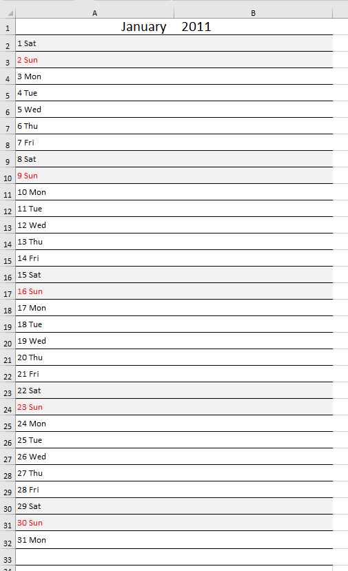
The image above shows a calendar that is dynamic meaning you choose year and month and the calendar instantly updates the dates accordingly.
There is a more advanced version here: Calendar – monthly view that lets you add events and more.
1.1 How the template works
Select a month and year. The cells (C2 and E2) are drop down lists. The calendar is instantly updated with dates. This makes it quick and easy to print months. You may have to adjust print area.
1.2 How I created the template
Adjust cell sizes
My calendar has seven columns and six rows filled with dates.
- Select the first seven columns
- Adjust width, I am using 128 px

- Select six rows
- Adjust height (90 px)
Create drop down lists
- Select cell C2
- Create a drop down list (Data validation)
- Select List
- In source field, type: January, February, March, April, May, June, July, August, September, October, November, December
Repeat with cell E2, in source field, type; 2011, 2012, 2013, 2014, 2015
Calculate start date
I created a second sheet "Calculation".

Formula in C4:
Cell range A1:A12 contains: January, February, March, April, May, June, July, August, September, October, November, December
Calendar formulas
- Select sheet1.
- Select cell A4, type in formula window: =Calculation!C4 + ENTER
- Select cell B4, type in formula window: =A4 +1 + ENTER.
- Select cell A5, type in formula window: =G4 +1 + ENTER
- Copy cell A5 and paste it down as far as needed.
- Select cell B4 and paste it to cell range B4:G9
Format cells
- Select sheet1
- Select cell range A4:G9
- Press with left mouse button on "Top Align" button (Home tab, excel 2007)
- Press with left mouse button on "Align text left" button (Home tab, excel 2007)
- Press CTRL + 1
- Press with left mouse button on "Number" tab
- Press with left mouse button on Category: Custom
- Type: D
- Press with left mouse button on OK
Create named range
- Create named range, named "month"
- In Referes to: field, type: =DATE(YEAR(Calculation!$C$4), MONTH(Calculation!$C$4)+1, 1)

- Select cell range A1:A12 in sheet "Calculation"
- Type months in name box
Conditional formatting
- Select sheet1
- Select cell range A4:G9
- Press with left mouse button on "Conditional formatting" button
- Press with left mouse button on "New Rule.."
- Press with left mouse button on "Use a formula to determine which cells to format"
- Type: =MONTH(A4)<>(MONTH(month))
- Press with left mouse button on "Format..." button
- Press with left mouse button on "Font" tab
- Select a color (grey)
- Press with left mouse button on OK!
- Press with left mouse button on OK!
1.3 Get excel calendar template
1.4 Week starts with monday
2. Monthly calendar template 2
I have created another monthly calendar template for you to get. Select a month and year in cells A1 and B1. They are drop down lists. The calendar is instantly updated with dates. This makes it quick and easy to print months. You may have to adjust print area.
2.1 How I created the template
Adjust column size
- Increase size of column A to 288 px.
- Increase size of column B to 288 px.
Adjust row sizes
- Select rows 1:33
- Adjust cell height to 30 px.
Create drop down lists
- Select cell A1
- Create a drop down list (Data validation)
- Select List
- In source field, type: January, February, March, April, May, June, July, August, September, October, November, December
Repeat with cell B1, in source field, type; 2011, 2012, 2013, 2014, 2015
Calculate start date
Formula in cell D1:
Hide formula in cell D1
- Select cell D1
- Press and hold CTRL and then press 1 once.
- Press with left mouse button on "Number" tab
- Press with left mouse button on "Custom" in Category window.
- Type ,,, in Type: field.
- Press with left mouse button on OK!
Calendar formulas
In cell A2:
In cell A3:
Copy cell A3 and paste into cell range A3:A32
Format cells
- Select cell range A2:A32
- Press with left mouse button on "Top Align" button (Home tab, excel 2007)
- Press with left mouse button on "Align text left" button (Home tab, excel 2007)
- Select font size 12
Conditional formatting - Highlight weekends
- Select cell range A2:B32
- Press with left mouse button on "Conditional formatting" button
- Press with left mouse button on "New Rule.."
- Press with left mouse button on "Use a formula to determine which cells to format"
- Type: =WEEKDAY($D$1+ROW(A1)-1, 2)>5
- Press with left mouse button on "Format..." button
- Press with left mouse button on "Fill" tab
- Select a color (grey)
- Press with left mouse button on OK!
- Press with left mouse button on OK!
Conditional formatting - Format sundays, font color to red
- Select cell range A2:B32
- Press with left mouse button on "Conditional formatting" button
- Press with left mouse button on "New Rule.."
- Press with left mouse button on "Use a formula to determine which cells to format"
- Type: =WEEKDAY($D$1+ROW(A1)-1, 2)=7
- Press with left mouse button on "Format..." button
- Press with left mouse button on "Font" tab
- Select a color (red)
- Press with left mouse button on OK!
- Press with left mouse button on OK!
Format cells
- Select cell A2:B2
- Press with left mouse button on top border button (Home tab)
- Press with left mouse button on bottom border button (Home tab)
- Press and hold with right mouse button on black dot in the right lower corner of cell B2
- Drag down to row 33
- Press with left mouse button on "Fill formatting only"
3. Calendar monthly view - Excel 365

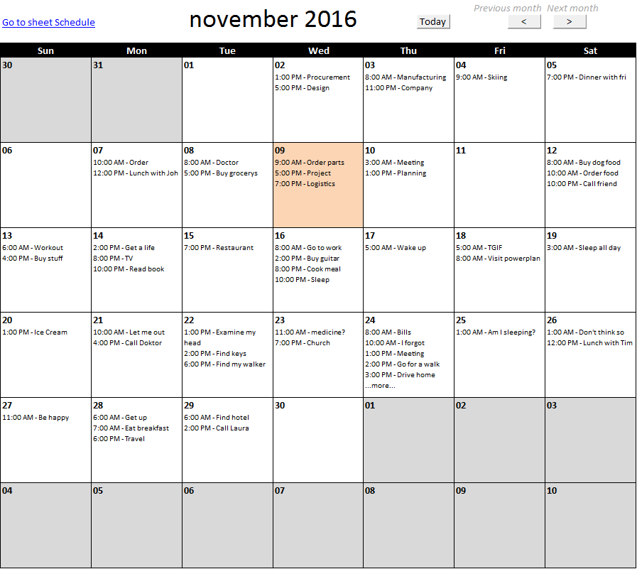
The image above demonstrates a calendar built for Excel 365, it doesn't contain any VBA macros. Everything is built on new Excel 365 functions and some Form Controls.
The calendar gets the information from an Excel Table located next to the calendar based on the displayed date in cell C2. You can change the date shown in cell C2 by pressing the left mouse button on the spin buttons next to year and month.

The first cell in each date box contains a formula, it spills data to the cells below automatically if needed. The formula returns a #SPILL! error if there are more data to show than rows.
Formula in cell B7:
Explaining formula in cell B7
Step 1 - Specify an absolute structured reference to an Excel Table named Table1
A cell reference to a column in an Excel Table is called a structured reference. When you copy a cell and paste to another cell the structured reference changes, in order to lock or create an absolute structured reference you need to use a colon and references before and after the colon.
A regular structured reference: Table1[Date and time]
An absolute structured reference: Table1[[Date and time]:[Date and time]]
Step 2 - Remove decimals or time from an Excel date and time value
The INT function removes the decimal part from positive numbers and returns the whole number (integer) except negative values are rounded down to the nearest integer.
Function syntax: INT(number)
INT(Table1[[Date and time]:[Date and time]])
becomes
INT({45231.5416666667; 45231.7083333333; 45232.3333333333; ... ; 2555})
and returns
{45231; 45231; 45232; ... ; 2555}
Step 3 - Remove decimals or time from an Excel date and time value
The equal sign lets you compare value to value in an Excel formula. You can also use it to compare values in an array, the result in both cases are boolean values TRUE or FALSE.
INT(Table1[[Date and time]:[Date and time]])=B6
becomes
{45231; 45231; 45232; ... ; 2555}=45228
and returns
{FALSE; FALSE; FALSE; ... ; FALSE}.
Step 4 - Filter values based on boolean values
The FILTER function extracts values/rows based on a condition or criteria.
Function syntax: FILTER(array, include, [if_empty])
FILTER(Table1[[Time and Title]:[Time and Title]],INT(Table1[[Date and time]:[Date and time]])=B6,"")
becomes
FILTER(Table1[[Time and Title]:[Time and Title]],{FALSE; FALSE; FALSE; ... ; FALSE},"")
and returns nothing "". All values are filtered out and the FILTER function returns #CALC! error, however, the third argument in the FILTER function lets you specify what to return if that happens.
In this case, "" nothing is returned which displays a blank cell.
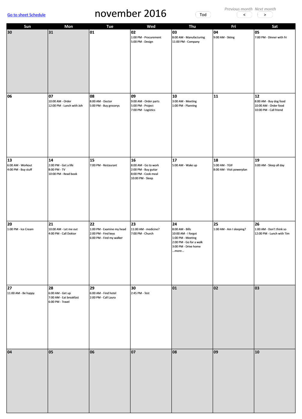
4. Calendar, monthly view - VBA
How easy is it to modify this for recurring tasks (weekdays, weekly, monthly, quarterly and yearly) and maybe show a monthly view? Times are less important than just showing what is due on what day.
I made a calendar shown below, monthly view. The picture is resized to fit this blog, press with left mouse button on to see the original size. This calendar is more advanced than the template I made year 2011.
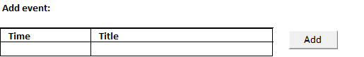
2.2. Add event
The form next to the calendar allows you to add events. Enter time and event name and then press with left mouse button on button "Add".
2.3. See all events on a specific date
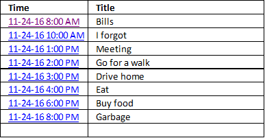
If there are more events on a single day than can be displayed, the last line tells you ...more.... See picture below for an example.
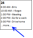
Select that cell and all events are shown in a table next to the calendar.
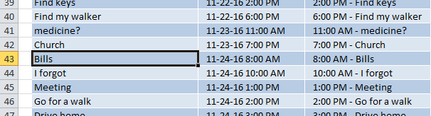
2.4. Edit event
You can easily edit or delete an event by press with left mouse button oning a link in column Time, see picture above. The link takes you to the record on sheet "Schedule", see picture below.
Here you can edit or delete the record as you please.
2.5. Change month - worksheets buttons
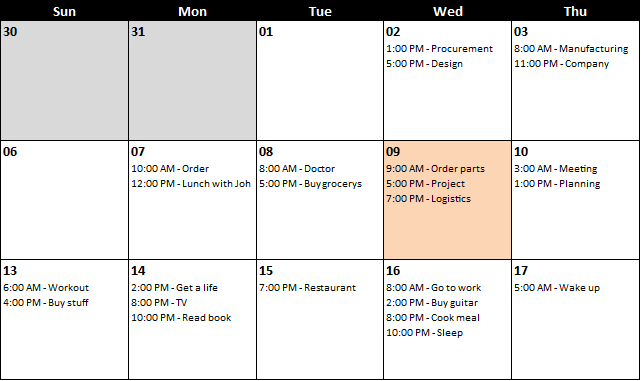
The buttons above the calendar lets you go to next or previous month, there is also a button that takes you to the current month, button "Today"

2.6. Conditional formatting
Days before and after selected month are grayed out. Current day is highlighted orange. The following picture shows you this.
2.7. Recurring events
The best I could do is creating a formula that calculates the upcoming recurring event. Events after that are not shown until the actual date has passed.
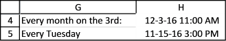
Monthly
Array formula in cell H4:
Explaining formula in cell H4
Step 1 - Calculate current date
The TODAY function returns today's date, it is a volatile function meaning it recalculates each time the worksheet is recalculated.
TODAY() returns 44357 formatted as 6/10/2021.
Step 2 - Calculate year
The YEAR function returns a number representing the year based on an Excel date.
YEAR(TODAY())
becomes
YEAR(44357)
and returns 2021
Step 3 - Calculate month
The MONTH function returns a number representing the relative position. For example, 1 is January, 2 is February, ..., 12 is December.
MONTH(TODAY())
becomes
MONTH(44357)
returns 6. June is the sixth month.
Step 4 - Calculate date next month
The DATE function returns a date based on a year, month, and day number.
DATE(YEAR(TODAY()), MONTH(TODAY())+1, 3)
becomes
DATE(2021, MONTH(TODAY())+1, 3)
becomes
DATE(2021, 6+1, 3)
becomes
DATE(2021, 7, 3)
and returns 44380 (7/3/2021).
Step 5 - Calculate date next month and time
DATE(YEAR(TODAY()), MONTH(TODAY())+1, 3)+11/24
becomes
44380 +11/24
and returns 44380.4583333333 (7/3/2021 11:00 AM).
Step 6 - Calculate date this month and time
DATE(YEAR(TODAY()), MONTH(TODAY()), 3)+11/24
Step 7 - Check if today is larger than 3
IF(DAY(TODAY())>3, DATE(YEAR(TODAY()), MONTH(TODAY())+1, 3)+11/24, DATE(YEAR(TODAY()), MONTH(TODAY()), 3)+11/24)
Weekly
Array formula in cell H5:
Daily
Array formula:
Anyone got a better idea?
2.8. Big version
This bigger version has 10 rows per day.
Calendar category
Table of Contents Excel monthly calendar - VBA Calendar Drop down lists Headers Calculating dates (formula) Conditional formatting Today Dates […]
Table of Contents Plot date ranges in a calendar Plot date ranges in a calendar part 2 Highlight events in […]
The image above demonstrates a calendar in Excel that allows you to: Add events. An event contains a date and […]
Templates category
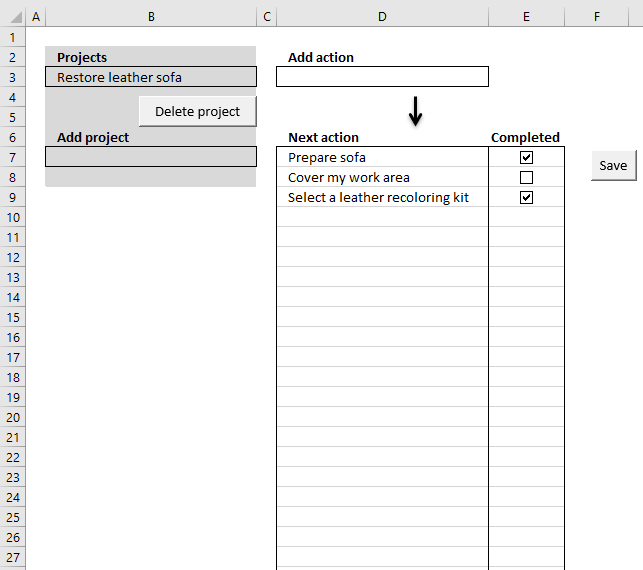
I am going to demonstrate a simple workbook where you can create or delete projects and add "next" actions to […]
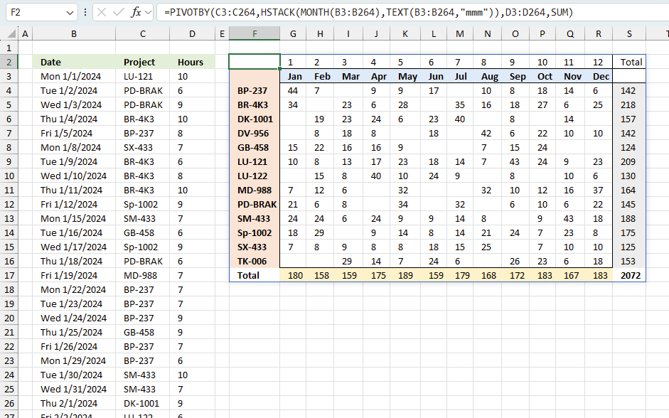
Tracking work hours across multiple projects can be challenging but Excel makes it easy with built-in functions. In this guide, […]
Excel categories
64 Responses to “Monthly calendar template”
Leave a Reply
How to comment
How to add a formula to your comment
<code>Insert your formula here.</code>
Convert less than and larger than signs
Use html character entities instead of less than and larger than signs.
< becomes < and > becomes >
How to add VBA code to your comment
[vb 1="vbnet" language=","]
Put your VBA code here.
[/vb]
How to add a picture to your comment:
Upload picture to postimage.org or imgur
Paste image link to your comment.
I have a calendar that is layed out like a monthly one with 7 days per week across and 5 weeks below, I have a list with event date and catagory, I am trying to get it to where I can use my drop down on the calendar seet for the catagory and have the items fill in on the dates per teh catagory, I have some catagories that have the same dates so I have 6 rows under each date I have it referanceing the date and tha catagory up top to the list to try to do the calendar. I can get it to work to a point some catagories will show through the whole month while others will omit the first week or 2 and or the last week or 2. My formula is
=IFERROR(IF(VLOOKUP(INDEX(Title, SMALL(IF($D$18=Datea, ROW(Datea)-MIN(ROW(Datea))+1, ""), ROW(A1))),Sheet2!$B$1:$G$200,6,FALSE)$C$1,"",INDEX(Title, SMALL(IF($D$18=Datea, ROW(Datea)-MIN(ROW(Datea))+1, ""), ROW(A1)))),"")
As a Aray
D18 is the date on the calendar that its looking for happens to be Tuesday January 17th 2011
Title = Sheet2!B1:B200
Datea = Sheet2!D1:D200
Column 6 has the catagories and $c$1 has a dropdown name list of the catagories to mathc against.
When going back and looking at my name referacnes it will change the referance values even if I have it locked as Sheet2!$B$1:$B$200 I have take out the names and put in the locked cells and move them down to like B27:B227
I would send my spreadsheet if i coudl for youto look at for better referance or at least a screen shot but I cant here and your contact me link comes up and Not Found.
Thanks for any help with this.
Oscar, You have probably for got more Excel that I expect to learn but your web site is a great resource. I'm not sure where to add this, so bear with me. Calendaring. I like this look but for simplicity "lists work as well. Beautification can come later. Here's the challenge. Private calendar, School Calendar and a work planning calendar all on seperate sheets in one work book. One additional sheet contains the "Calendar year" starting Jan1 2013. I use "Weeknum" to extract the week number, then use "countif" to determine how many activities exisit on the various sheets for a given week. Now I'm stuck, I'm scared of VBA because I'm not well versed in the tool. Ideally, I would like a column for the week number and then "vlookup" and display all the dates and descriptions of what is happening during that week from all the various sheets. This involves adding rows. I don't see a formula for that. Then the second week, third week.... Does this make sense? Could you point me in the right direction? Further limited by excel2003 (2010 should arrive sometime this year.) Thanks
Rich,
I am not sure if this is exactly what you are looking for:
I am using random letters.
Get the Excel *.xls file
https://www.get-digital-help.com/wp-content/uploads/2011/01/Combine-Calendars.xls
Is there a way to add more years? Possibly to 2020 or further?
Same question as Chris D above, how can we add additional years?
This is the cleanest calendar template I have seen yet and sure would like to continue using it.
[…] Monthly calendar template in excel […]
[…] Monthly calendar template in excel […]
Oscar, I was working on your monthly calendar template in Excel. I am using Office 365 ProPlus Excel 2013. have any of the formulas changed since you created? I am getting an #NAME? error on my Sheet 1 all the formulas and Calculation sheet C4.
[…] resized to fit this blog, Press with left mouse button to see the original size. This calendar is more advanced than the template I made year […]
Excellent, excellent job Mr. Oscar !!!
Diana,
thank you!
Thankyou Oscar,
I am very impressed with your Excel examples. The one that tops it all for me was your detailed Pivot Table - a masterclass...
Regards,
Ray
Thank you, Ray.
Happy you like it.
I do not know why the hyperlink in column J sheet Monthly view does not work(?) please help. Thanks
Hung,
You are right, thanks for telling me.
My blog (WordPress) has changed the name of the workbook when I uploaded the file, the hyperlink function uses another workbook name and that won't work.
Anyway, I have uploaded a new workbook and this time it seems to work.
Sorry I don't know how to use Recurring event. Please help. Thanks
Monthly formula:
=IF(DAY(TODAY())>3, DATE(YEAR(TODAY()), MONTH(TODAY())+1, 3)+11/24, DATE(YEAR(TODAY()), MONTH(TODAY()), 3)+11/24)
Change the bolded numbers above to select a day in a month. The example above uses the 3rd in every month. 11/24 is 11 AM. A day has 24 hours.
Weekly formula:
=TODAY()+IF(WEEKDAY(TODAY())<=3, 3-WEEKDAY(TODAY()), (10-WEEKDAY(TODAY())))+15/24
Change number 3 above to select a weekday, 1 is Sunday, 2 is Monday and so on. 15/24 is 3 pm.
The daily formula is self explanatory.
To use a recurring event, go to sheet schedule and select a cell in column "Day and Time" on an event you want to recur. Change the value to the desired formula.
wow, I got it :) thanks a lot
one small thing need to change in macro Add Event: row 5 to row 6
Worksheets("Schedule").Range("B" & Lrow) = ActiveSheet.Range("N5")
Worksheets("Schedule").Range("C" & Lrow) = ActiveSheet.Range("M5")
ActiveSheet.Range("M5:N5") = ""
Hung,
Thanks. There is a new file attached.
This is so helpful! I am using it as a sprint planning calendar to track different work streams! THANK YOU!
Gina,
Thank you for commenting.
Hi, Any chance I can get the template as in this page.. It is all very much beyond me, and I really like what you have some here. Please
Gary
I am happy you like it, there is a file link at the end of this post.
Thank you so much for this great and very helpful calendar. Is there a way to have a recurring event as birthday reminder using either an Excel function as in your example or obtained from a list of dates and names?
(Cont'd) Also, is it able to add repeated recurring events such as paydays (every 2 weeks on Friday, Saturday work every 5 weeks...).
Thanks and best wishes!
Hi Oscar, this was very helpful for me as well and have implemented these calendars in my workbook! Do you know if there is a way to show more than 5 items on a day in the calendar view, maybe 10 lines?
Meggan,
Yes, Excel file:
https://www.get-digital-help.com/wp-content/uploads/2016/11/Calendar-monthly-view3-meggan.xlsm
Thank you so much!
I forgot to change the macros and event code.
Here is a new file:
https://www.get-digital-help.com/wp-content/uploads/2016/11/Calendar-monthly-view3-meggan-1.xlsm
I believe it is working better now.
Oscar, Thank you for the template!
Question: some of my longer events are truncated. "Pancake Breakfast" shows up as "8:00am - Pancake Breakfas" it seems there is a character limit somewhere in the code but I can't find it.
Any ideas?
Also, I'd love to have the date, and the time in separate columns. That way for time I could leave it blank, OR I could use 'times' like "All Day" or "Afternoon".
Mike Ver Duin
Thank you
Question: some of my longer events are truncated. "Pancake Breakfast" shows up as "8:00am - Pancake Breakfas" it seems there is a character limit somewhere in the code but I can't find it.
Any ideas?
Yes, change value 25 in this line: result = result & Left(ReturnCol.Cells(i), 25) & vbNewLine
Function Lookup_concat(SearchDate As String, _ SDate As Range, ReturnCol As Range) Dim i As Long Dim result As String For i = 1 To SDate.Cells.CountLarge If Int(SDate.Cells(i)) = SearchDate Then If j >= 5 Then result = result & "...more..." Exit For End If result = result & Left(ReturnCol.Cells(i), 25) & vbNewLine j = j + 1 End If Next i Lookup_concat = Trim(result) End FunctionHi Oscar,
Can you convert this to use as a yearly and monthly calendar
Thanks in advance
Michelle,
Perhaps this is working for you?
https://www.get-digital-help.com/yet-another-excel-calendar/
Hi! This worksheet works perfectly!
However, can I check how do I modify the formulas such that I can define a start and end date to a certain event, and it will populate for each of the dates involved?
Thanks in advance!
Chloe
Check out this calendar:
https://www.get-digital-help.com/highlight-events-in-a-calendar/
Thanks for the alternative link!
But what I'm hoping to look for is to populate out the Events name in my calendar view based on start and end date, instead of highlighting the cells using conditional formatting. How should I embed the formula in my table's look up formula? :)
Chloe
I would suggest that you enter the date and time for the event multiple times in the table, however, only the date will differ. That way you will get the event one each date.
The calendar uses the following UDF to get the events, if you want to customize it:
Function Lookup_concat(SearchDate As String, _ SDate As Range, ReturnCol As Range) Dim i As Long Dim result As String For i = 1 To SDate.Cells.CountLarge If Int(SDate.Cells(i)) = SearchDate Then If j >= 5 Then result = result & "...more..." Exit For End If result = result & Left(ReturnCol.Cells(i), 25) & vbNewLine j = j + 1 End If Next i Lookup_concat = Trim(result) End FunctionHi! Thanks for the reply! Have tried the method to key in date by date but this is rather time consuming on the user's end as some events can span across months.
Is there a way to tweak the form input such that I can just key in start and end date, then this will automatically populate into the data table per individual dates?
Thanks heaps!
Hi there Oscar,
I've recently started working in an office environment and I'm having to seriously step up my Excel 2016 knowledge.
What I'm aiming to do is design a calendar I can use as a daily checklist. It's a simple as this:
Each day needs to contain 9 cells, with borders, with items I can have reoccur from Monday to Friday. Each cell relates to a task. To show the task has been successfully completed I change the cell colour from white to green.
To stick with current checklist document trends, it would also be very helpful to be able to have each individual month displayed within a single page instead of a single page with a month changing menu.
I've opened your 10 Row Monthly Calendar, and tried applying weekly reoccuring events to no success. When i edit the 3,3 in:
=TODAY()+IF(WEEKDAY(TODAY())<=3,3-WEEKDAY(TODAY()),(10-WEEKDAY(TODAY())))
to 4,4 it does not change the event to a Wednesday and it does not reoccur on every Tuesday within the calendar when copied and pasted into the 'Date and Time' column of the 'Schedule' page. I have removed the time portion of the equation as I've changed the date format to only display the day as that's all need to know. I'm going to attribute this to my lack of understanding of the program.
There is the potential to need to add more cells to each day as more tasks need to be added to the calendar. Are you able to tell me how to edit to add more cells? There will be no variability in the number of tasks each day.
I'm so lost and I am really unsure of where to begin. Can you help?
Is there a way to add additional content in the schedule that will show in the monthly view?
How is the Lookup_concat function being added to every "date" on the calendar? I have modified the Schedule Table slightly, and want to update the function on all the calendar days, how would that be accomplished?
The UDF looks like this in cell B6:
=Lookup_concat(B6,Table1[Date and time],Table1[Time and Title])
Why don't you try out the workbook and check it out yourself?
The UDF VBA Code
Function Lookup_concat(SearchDate As String, _
SDate As Range, ReturnCol As Range)
Dim i As Long
Dim result As String
For i = 1 To SDate.Cells.CountLarge
    If Int(SDate.Cells(i)) = SearchDate Then
        If j >= 5 Then
            result = result & "...more..."
            Exit For
        End If
        result = result & Left(ReturnCol.Cells(i), 25) & vbNewLine
        j = j + 1
    End If
Next i
Lookup_concat = Trim(result)
End Function
I have modified the Schedule Table slightly, and want to update the function on all the calendar days, how would that be accomplished?
Have you inserted a new column to the Schedule table? Can you explain in greater detail?
Hello
This is a very useful and wonderful template, i have been trying to use this to suit my requirements but not succesful
I would like to add more 2 columns after the Time and Title Columns in the Schedule Sheet and the data in these columns should reflect in the calendar view , i have been trying to do nake changes but no success, could you kindly help me out this
Thanks a ton in advance
Rajesh
Rajesh,
Concatenate the two columns in the Title column, like this:
=A2&B2
You don't need to add additional VBA code to your workbook.
Hi,
Wonderful calendar spreadsheet. I am trying change the name of the file but seesm to "break the hyperlinks. Is there a simple way to update the links. Edit hyperlink is greyed out when I press with right mouse button.
Brent
Brent,
thank you.
I am trying change the name of the file but seems to "break the hyperlinks. Is there a simple way to update the links. Edit hyperlink is greyed out when I press with right mouse button.
Yes, you need to change the links in the formulas.
Array formula in cell J6:
=IFERROR(HYPERLINK("[Calendar-monthly-view3.xlsm]Schedule!$B$"&MATCH(SMALL(IF('Monthly view'!$K$3=INT(Table1[Date and time]),Table1[Date and time],""), ROW(A1)), Table1[Date and time],0)+2, SMALL(IF('Monthly view'!$K$3=INT(Table1[Date and time]), Table1[Date and time], ""), ROW(A1))), "")
See the bolded part above, don't forget to enter the formula as an array formula after you changed the formula.
Now copy cell J6 and paste as far as needed to cells below.
Hi, Oscar
This posting, along with the others related to calendars, are awesome! The discussions also answered many of my questions.
I have a question regarding text colour coding for different events on the same day in the Monthly view. I tried conditional formatting and find and replace, but neither worked. The former colours all the events the same, and the latter is unable to find the text to replace.
What would be the best way to approach this in Excel 2010? Thank you.
Christine
Oh yes, this is also something I'm curious about. I am hoping to be able to change the color of the text by person (ie, me in red, my husband in blue, my daughter in purple, etc. This way I can see whose event is happening at a particular time on a date. Is there a way for each cell to be separate, so these colors can be conditionally formatted, instead of it being concatenated into a large merged cell?
Thanks, this is a great calendar!
Zuania,
Not at the moment, I need to rebuild the macro that populates the cells in order to make it work with conditional formatting.
Hello! I am also interested in color coding for different types of events. Is there an updated version of this calendar with that functionality? Thanks so much!
I'm trying to try out this form. It's not working as I don't see the file link as for other forms on here. Am I doing something wrong?
Really simple, efficient and impressive. Thanks for this!
Tri,
thank you!
Hi When I enable content the date and time field displays as t:01 as in t:01 AM - Skiing without the date. Is there a fix for this? Thanks!
Oscar,
I am new to excel VBA macros. This is the exact calendar i need for my project but need to expand on it.
Can you please answer the following?
#1 how do i duplicate the title column on sheet 2(Schedule) cell D2?
#2 how do i add an color drop down list to reflect on the given date/time/title column?
#3 how can i add a master view and single view button of the selected titles on the calendar? that allows me to show only the selected from a drop down.
I appreciate your feedback!
How can one go to the current day when opening the book and is it possible to have a form with pending notices?
Is it possible to take outlet calendar and pull addresses in order from first day of month to last day of month to create a to and from list? And result travel log
Hi Oscar,
Is there a way to apply a filter to this calendar? Meaning on the schedule table, there is one more column called "Type" which have 2 options i.e. "Work", "Non-Work"
A dropdown list of "Type" created at the Monthly view sheets. The information on the calendar to change based on the dropdown list value
Thank you
i use the following formula for the filter. but its giving an error #VALUE!
=@Lookup_concat(B06,FILTER(Table1[Date and Time],Table1[Type]="Work"),FILTER(Table1[Time and Title],Table1[Type]="Work"))
how can i get this code
I have added and OPERATOR name to the "add event" schedule table.
Is there a way I can update the calendar locate_concat function and the list to only populate the result if the OP name = a certain field or drop down?
Id like to see the calendar with all my ops but also "filter" the schedule based on a selected op. Any guidance would be great
This is fantastic, thanks for sharing this!!
ReadyExcelFiles.com provides over 10,000+ ready-to-use, fully editable Excel worksheets designed to make work easier and faster for individuals and businesses across the United States. Our Excel files are created to support everyday professional needs, from finance and accounting to project tracking, inventory management, and business reporting.
Each worksheet is simple to use, professionally formatted, and customizable to fit your specific workflow. Whether you’re a small business owner, freelancer, student, or corporate professional, our Excel solutions help reduce manual effort and improve productivity.
With ReadyExcelFiles.com, you don’t need to build spreadsheets from scratch—
just download, edit, and get to work