Compare the performance of your stock portfolio to S&P 500 using Excel
Table of Contents
1. Compare the performance of your stock portfolio to S&P 500 using Excel

By comparing your stock portfolio performance to index S&P500 you know if the time you spent on analyzing companies paid off. In fact, Warren Buffet recommends investing in an SP500 index fund if you have no knowledge of investing in the stock market. Let's see if your portfolio beats S&P500 over time.
In previous posts a few years ago I explained how to use NAV units to calculate stock portfolio performance. I am going to use Net Asset Value based on units for a fictional stock portfolio in this article.
- Automate net asset value (NAV) calculation on your stock portfolio (vba)
- Calculate your stock portfolio performance with Net Asset Value based on units
Get data
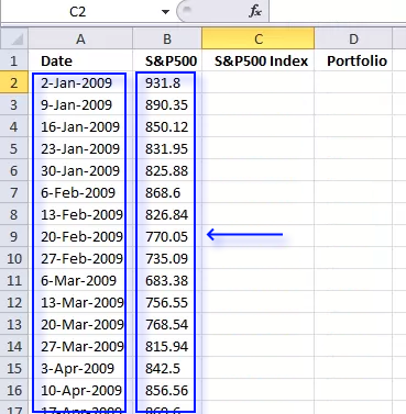
We need monthly data from both the stock portfolio and the S&P 500. First get historical weekly prices from Yahoo Finance. Copy and paste dates and prices to a new sheet in your workbook.
Calculate stock portfolio performance
The Excel workbook attached to Automate net asset value (NAV) calculation on your stock portfolio (vba) can automatically calculate portfolio performance using NAV (net asset value). You can't base portfolio perfomance on account balance.
Open the Excel workbook and insert the last date to each week and then press "Update" button. Make sure dates (col A) are sorted.

Copy values to a new table
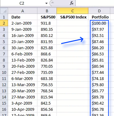
- Copy "NAV per share" data from the "Transactions" sheet and corresponding dates.
- Select the new sheet containing the yahoo S&P 500 prices you geted.
- Paste "NAV per share" data and corresponding dates.
Indexing S&P 500 data

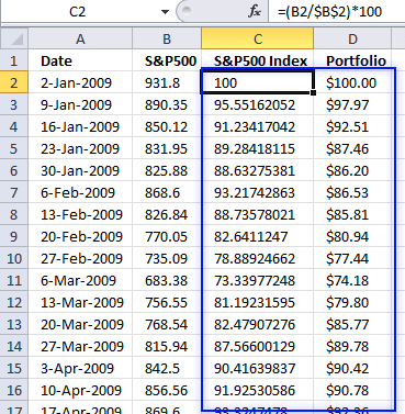
Index SP500 to 100. This makes it a lot easier to compare performance relative to your stock portfolio. Both your stocks and the index must start at the same value, I am going for 100 which is often used.
Formula in cell C2:
Copy formula to cells below as far as needed.
Explaining formula in cell C2
Step 1 - Divide first value with current value
The forward slash is an arithmetic operator that lets you divide a number with another number. The first cell reference B2 is a relative cell reference that changes when you copy the cell and paste to cells below.
The second cell reference is an absolute cell reference that is locked to cell B2 all the time (except if you insert rows or columns). This allows us to divide the corresponding value on the same row with the first value and calculating the outcome in percentage date by date.
B2/$B$2
becomes
931.8/931.8
and returns 1.
Step 2 - Multiply with 100
The parentheses let you control the order of operations, we want it to do the division before we multiply with 100.
(B2/$B$2)*100
becomes
1*100
and returns 100.
Create a chart showing portfolio and S&P 500 performance
- Select values in column C and D.
- Go to tab "Insert" on the ribbon.
- Press with left mouse button on "Line chart" button.
2. Tracking a stock portfolio in Excel (auto update)
Question:
I found a question here about tracking a stock portfolio. He would like to automatically create an overview table with a unique stock symbol per row. He also wants the range extended down to include new rows as they become valid.
Example,
Answer:
Sheet1
![]()
Sheet2
![]()
Create named ranges
- Select tab "Formulas" on the ribbon
- Press with left mouse button on "New..." button
- Type
Symbol
in Name: bar
- Type formula:
=Sheet1!$A$2:INDEX(Sheet1!$A:$A, COUNTA(Sheet1!$A:$A))
in "Refers to:" bar
- Press with left mouse button on Close button
Repeat above instructions with following names and formulas:
Type - =Sheet1!$B$2:INDEX(Sheet1!$B:$B, COUNTA(Sheet1!$B:$B))
Shares - =Sheet1!$C$2:INDEX(Sheet1!$C:$C, COUNTA(Sheet1!$C:$C))
Price - =Sheet1!$D$2:INDEX(Sheet1!$D:$D, COUNTA(Sheet1!$D:$D))
Array formulas
Array formula in cell A2, sheet 2:
Copy cell A2 and paste down as far as needed. This formula creates uniue distinct symbols. Read this post: How to extract a unique distinct list from a column for a formula explanation.
Array formula in cell B2, sheet 2:
Copy cell B2 and paste down as far as needed.
Get excel file
Tracking a stock portfolio.xlsx
(Excel 2007 -2010 Workbook *.xlsx)
Pivot table - Semi auto update
You can also convert the range in sheet1 to a table and then create a pivot table with data from table. The table includes new rows automatically. Unfortunately the pivot table does not. Press with right mouse button on anywhere on pivot table and press with left mouse button on Refresh when new rows are added.
![]()
The question is how to subtract sold shares from bought shares in a pivot table?
3. Tracking a stock portfolio #2
In this section we are going to calculate cost basis and returns. The calculations are simplified, commissions, stock splits and dividends are removed from calculations.
In the first post we created dynamic ranges.

We also identified accumulated stocks and the number of shares. I have now added cost basis and returns.

Excel formula in cell C2:
Copy cell C2 and paste down as far as needed.
How this formula works in cell C2
Step 1 - Calculate total cost you paid
=IF(A2<>"", (SUMPRODUCT((A2=Symbol)*(Type="Buy")*Shares*Price)-SUMPRODUCT((A2=Symbol)*(Type="Sell")*Shares*Price))/(SUMPRODUCT((A2=Symbol)*(Type="Buy")*Shares)-SUMPRODUCT((A2=Symbol)*(Type="Sell")*Shares)), "")
SUMPRODUCT(array1, array2, )
Returns the sum of the products of the corresponding ranges or arrays
SUMPRODUCT((A2=Symbol)*(Type="Buy")*Shares*Price)
becomes
SUMPRODUCT((F={F, MSFT, MSFT, F, GOOG, MSFT, GOOG, GOOG, GOOG}))*({Buy, Buy, Buy, Buy, Sell, Sell, Buy, Buy, Sell}=Buy)*{100, 100, 50, 100, 25, 50, 10, 100, 200}*{12, 25, 28, 16, 550, 24, 500, 500, 550})
becomes
SUMPRODUCT(({TRUE, FALSE, FALSE, TRUE, FALSE, FALSE, FALSE, FALSE, FALSE}))*({TRUE, TRUE, TRUE, TRUE, FALSE, FALSE, TRUE, TRUE, FALSE})*{100, 100, 50, 100, 25, 50, 10, 100, 200}*{12, 25, 28, 16, 550, 24, 500, 500, 550})
becomes
SUMPRODUCT({1200, 0, 0, 1600, 0, 0, 0, 0, 0}) returns 2800.
Step 2 - Calculate total amount you sold
=IF(A2<>"", (SUMPRODUCT((A2=Symbol)*(Type="Buy")*Shares*Price)-SUMPRODUCT((A2=Symbol)*(Type="Sell")*Shares*Price))/(SUMPRODUCT((A2=Symbol)*(Type="Buy")*Shares)-SUMPRODUCT((A2=Symbol)*(Type="Sell")*Shares)), "")
SUMPRODUCT((A2=Symbol)*(Type="Sell")*Shares*Price)
becomes
SUMPRODUCT({0, 0, 0, 0, 0, 0, 0, 0, 0}) returns 0.
Step 3 - Calculate accumulated shares
=IF(A2<>"", (SUMPRODUCT((A2=Symbol)*(Type="Buy")*Shares*Price)-SUMPRODUCT((A2=Symbol)*(Type="Sell")*Shares*Price))/(SUMPRODUCT((A2=Symbol)*(Type="Buy")*Shares)-SUMPRODUCT((A2=Symbol)*(Type="Sell")*Shares)), "")
(SUMPRODUCT((A2=Symbol)*(Type="Buy")*Shares)-SUMPRODUCT((A2=Symbol)*(Type="Sell")*Shares
becomes
SUMPRODUCT({100, 0, 0, 100, 0, 0, 0, 0, 0}) - SUMPRODUCT({0, 0, 0, 0, 0, 0, 0, 0, 0})
and returns 200.
Step 4 - Calculate cost basis
=IF(A2<>"", (SUMPRODUCT((A2=Symbol)*(Type="Buy")*Shares*Price)-SUMPRODUCT((A2=Symbol)*(Type="Sell")*Shares*Price))/(SUMPRODUCT((A2=Symbol)*(Type="Buy")*Shares)-SUMPRODUCT((A2=Symbol)*(Type="Sell")*Shares)), "")
becomes
=IF(A2<>"", (2800-0)/200, "") returns 14 in cell C2.

Excel formula in cell D2
Copy cell D2 and paste down as far as needed.
How this formula works in cell D2
Step 1 - Calculate average price you paid per share
=IF(A2<>"", (IFERROR(SUMPRODUCT(--(A2=Symbol), --("Sell"=Type), Price, Shares)/SUMPRODUCT(--(A2=Symbol), --("Sell"=Type), Shares), 0)-IFERROR(SUMPRODUCT(--(A2=Symbol), --("Buy"=Type), Price, Shares)/SUMPRODUCT(--(A2=Symbol), --("Buy"=Type), Shares), 0))*(MIN(SUMPRODUCT(--(A2=Symbol), --("Sell"=Type), Shares), SUMPRODUCT(--(A2=Symbol), --("Buy"=Type), Shares))), "")
(IFERROR(SUMPRODUCT(--(A2=Symbol), --("Sell"=Type), Price, Shares)/SUMPRODUCT(--(A2=Symbol), --("Sell"=Type), Shares), 0)
returns 0.
Step 2 - Calculate average selling price
=IF(A2<>"", (IFERROR(SUMPRODUCT(--(A2=Symbol), --("Sell"=Type), Price, Shares)/SUMPRODUCT(--(A2=Symbol), --("Sell"=Type), Shares), 0)-IFERROR(SUMPRODUCT(--(A2=Symbol), --("Buy"=Type), Price, Shares)/SUMPRODUCT(--(A2=Symbol), --("Buy"=Type), Shares), 0))*(MIN(SUMPRODUCT(--(A2=Symbol), --("Sell"=Type), Shares), SUMPRODUCT(--(A2=Symbol), --("Buy"=Type), Shares))), "")
IFERROR(SUMPRODUCT(--(A2=Symbol), --("Buy"=Type), Price, Shares)/SUMPRODUCT(--(A2=Symbol), --("Buy"=Type), Shares)
returns 14.
Step 3 - Multiply with bought or sold shares
=IF(A2<>"", (IFERROR(SUMPRODUCT(--(A2=Symbol), --("Sell"=Type), Price, Shares)/SUMPRODUCT(--(A2=Symbol), --("Sell"=Type), Shares), 0)-IFERROR(SUMPRODUCT(--(A2=Symbol), --("Buy"=Type), Price, Shares)/SUMPRODUCT(--(A2=Symbol), --("Buy"=Type), Shares), 0))*(MIN(SUMPRODUCT(--(A2=Symbol), --("Sell"=Type), Shares), SUMPRODUCT(--(A2=Symbol), --("Buy"=Type), Shares))), "")
MIN(SUMPRODUCT(--(A2=Symbol), --("Sell"=Type), Shares), SUMPRODUCT(--(A2=Symbol), --("Buy"=Type), Shares))
returns 0.
Step 4 - Calculate returns
=IF(A2<>"", (IFERROR(SUMPRODUCT(--(A2=Symbol), --("Sell"=Type), Price, Shares)/SUMPRODUCT(--(A2=Symbol), --("Sell"=Type), Shares), 0)-IFERROR(SUMPRODUCT(--(A2=Symbol), --("Buy"=Type), Price, Shares)/SUMPRODUCT(--(A2=Symbol), --("Buy"=Type), Shares), 0))*(MIN(SUMPRODUCT(--(A2=Symbol), --("Sell"=Type), Shares), SUMPRODUCT(--(A2=Symbol), --("Buy"=Type), Shares))), "")
becomes
=IF(A2<>"", (0-14)*0) returns 0
Final notes
I am not telling you to sell or buy any stock, this is just an example.
I hope I got all calculations right.
Get excel file
Tracking-a-stock-portfolio2.xlsx
(Excel 2007 -2010 Workbook *.xlsx)
Stock portfolio category
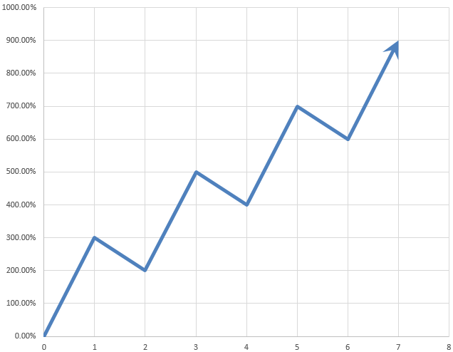
Table of Contents Automate net asset value (NAV) calculation on your stock portfolio Calculate your stock portfolio performance with Net […]
Excel categories
7 Responses to “Compare the performance of your stock portfolio to S&P 500 using Excel”
Leave a Reply
How to comment
How to add a formula to your comment
<code>Insert your formula here.</code>
Convert less than and larger than signs
Use html character entities instead of less than and larger than signs.
< becomes < and > becomes >
How to add VBA code to your comment
[vb 1="vbnet" language=","]
Put your VBA code here.
[/vb]
How to add a picture to your comment:
Upload picture to postimage.org or imgur
Paste image link to your comment.
Thanks for making a more elaborate answer to the question I originally posted on SuperUser. Using INDEX and COUNTA to create an auto updating named range is something I had originally considered.
However, in the end I had to resort to writing a VSTO add-in to get all the behavior I wanted. I kept running into even more complex problems that I couldn't solve in excel natively.
Hi Oscar,
I have a similar question, but my problem size is 580,526 products. which i need to consolidate. I used the same formula mentioned above, the computational time is 5 hours and still running. Suggest something else.
Regards,
Chetan
Thanks for the blog. nice 1. it's what I was looking for
Bhavik.
Bhavik,
Thank you!
Just to say thank you for this article, it's exactly what i have been looking for.
Duncan
Hi Oscar,
I have a similar question, but my problem size is 580,526 products. which i need to consolidate. I used the same formula mentioned above, the computational time is 5 hours and still running. Suggest something else.
Regards,
Chetan
Hi Oscar,
Thank you for the information on your website.
Actually i have a question please.
For a SELL position, why do you add the 'Total Stock Value' to the 'Balance'. The security is already sold and the proceeds have already been added to the 'Balance'. In a SELL situation, the 'Total Stock Value' should be 0, right?
Thanks,
Danen