A Comprehensive Guide to Splitting Text in Excel
This blog article describes how to split strings in a cell with space as a delimiting character, like Text to columns. Text to columns separates the contents of one cell into separate columns.
I present here four different formulas that does the job, I recommend example 3 or example 4. Short and easy to understand.
Table of Contents
- Split words in a cell - blank as a delimiting character
- Split words in a cell - any delimiting character(s)
- Split words in a cell - Excel 365 formula
- Split words in a cell - Excel 365 formula - any delimiting character(s)
- Split words in a cell - Rick Rothstein's formula
- Split words in a cell - Rick Rothstein's formula - Any delimiting character(s)
- Split words in a cell - FILTERXML function - any a delimiting character
- Use text qualifiers to make text to columns conversion easier - UDF
- Get Excel file
- Extract values between two given delimiting strings
- Extract text between words - UDF
- Split words in a cell range into a cell each [UDF]
- Split words in a cell range into a cell each - Excel 365
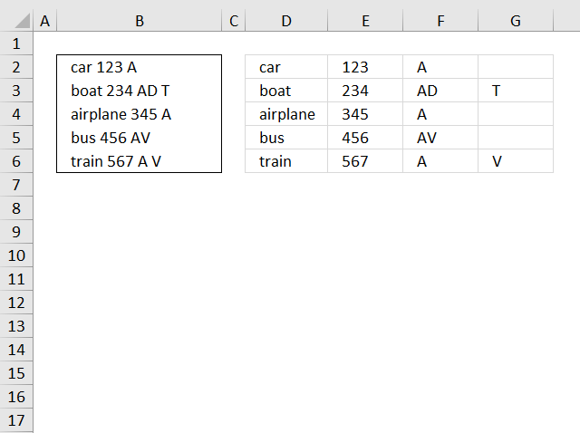
1. Blank as a delimiting character - array formula
Array formula in cell D1:
To enter an array formula, type the formula in a cell then press and hold CTRL + SHIFT simultaneously, now press Enter once. Release all keys.
The formula bar now shows the formula with a beginning and ending curly bracket telling you that you entered the formula successfully. Don't enter the curly brackets yourself.
Copy cell D2 and paste to cell range D2:G6.
Explaining formula in cell D1
Step 1 - Split characters in a cell into an array
The MID function returns a substring from a string based on the starting position and the number of characters you want to extract. The ROW function returns an array from 1 to 99.
MID(" "&$B2&" ", ROW($1:$99), 1)
becomes
MID(" car 123 A ", {1; 2; 3; 4; 5; 6; 7; 8; 9; 10; 11; ... ; 99}, 1)
and returns this array:
{" "; "c"; "a"; "r"; " "; "1"; "2"; "3"; " "; "A"; ... ; ""}
Step 2 - Search for a blank as a delimiting character and return position
The SEARCH function returns the number of the character at which a specific character or text string is found reading left to right (not case-sensitive), if string is not found the function returns an error value. The ISERROR function returns TRUE if the value is an error.
The IF function has three arguments, the first one must be a logical expression. If the expression evaluates to TRUE then one thing happens (argument 2) and if FALSE another thing happens (argument 3). If the ISERROR function returns FALSE the function returns the corresponding row number.
The SMALL function then returns the k-th smallest value in the array based on the column function and a relative cell reference that changes when the cell is copied to the next cell. This makes the formula return a new value in each cell.
SMALL(IF(ISERROR(SEARCH(MID(" "&$B2&" ", ROW($1:$99), 1), " ")), "", ROW($1:$99)), COLUMN(A1))
becomes
SMALL({1; ""; ""; ""; 5; ""; ""; ""; 9; ""; ... ; 99}, COLUMN(A1))
and returns 1.
Step 3 - Calculate length argument in mid function
SMALL(IF(ISERROR(SEARCH(MID(" "&$B2&" ", ROW($1:$99), 1), " ")), "", ROW($1:$99)), COLUMN(A1)+1)-SMALL(IF(ISERROR(SEARCH(MID(" "&$B2&" ", ROW($1:$99), 1), " ")), "", ROW($1:$99)), COLUMN(A1)))
SMALL({1; ""; ""; ""; 5; ""; ""; ""; 9; ""; ... ; 99}, 2)-SMALL({1; ""; ""; ""; 5; ""; ""; ""; 9; ""; ... ; 99}, 1)
becomes
5-1 equals 4.
Step 4 - Filter word
=MID(" "&$B2&" ", SMALL(IF(ISERROR(SEARCH(MID(" "&$B2&" ", ROW($1:$99), 1), " ")), "", ROW($1:$99)), COLUMN(A1)), SMALL(IF(ISERROR(SEARCH(MID(" "&$B2&" ", ROW($1:$99), 1), " ")), "", ROW($1:$99)), COLUMN(A1)+1)-SMALL(IF(ISERROR(SEARCH(MID(" "&$B2&" ", ROW($1:$99), 1), " ")), "", ROW($1:$99)), COLUMN(A1)))
becomes
=MID(" "&$B2&" ", 1, 4)
becomes
MID(" car 123 A ", 1, 4)
and returns "car" in cell D2.
2 Any delimiting character - array formula

The formula in cell D2 in the image above shows how to split a text string using a comma but you can use any number of characters if you like.
For example, replace this "," with the delimiting characters you want to use. Perhaps you want to use three characters example: " | ", make sure you add double quotes before and after. Replace all instances of "," with " | " in the formula below.
3. Blank as a delimiting character - Excel 365 formula

Update! The new TEXTSPLIT function is built for this scenario.
Excel 365 formula in cell D2:
Deprecated: Function get_page_by_title is deprecated since version 6.2.0! Use WP_Query instead. in /var/www/html/get-digital-help.com/public_html/wp-includes/functions.php on line 6031
The TEXTSPLIT function splits a string into an array based on delimiting values.
Function syntax: TEXTSPLIT(Input_Text, col_delimiter, [row_delimiter], [Ignore_Empty])
Old formula
The formula in cell D2 is almost identical to the one in example 1, however, the Excel 365 LET function shortens the formula considerably. The only thing that changed is that I am using the SEQUENCE function instead of the ROW function. The SEQUENCE function works with smaller appropriately sized arrays which makes this formula more efficient.
The formula above is entered as a regular formula and it works only in Excel 365.
4 Comma as a delimiting character - Excel 365 formula

The image above demonstrates a formula that splits strings using a comma, however, you can use whatever character or characters you want.
Update!
The new TEXTSPLIT function is built for this scenario.
Excel 365 formula in cell D2:
Deprecated: Function get_page_by_title is deprecated since version 6.2.0! Use WP_Query instead. in /var/www/html/get-digital-help.com/public_html/wp-includes/functions.php on line 6031
The TEXTSPLIT function splits a string into an array based on delimiting values.
Function syntax: TEXTSPLIT(Input_Text, col_delimiter, [row_delimiter], [Ignore_Empty])
Old formula
Replace every instance of "," in the formula below with the string you want as a delimiting character. Make sure you use double quotes before and after. For example, " | ".
The formula above is entered as a regular formula and it works only in Excel 365.
5. Example 3 - Text to columns with a blank as a delimiting character

This is Rick Rothstein's formula, read his comment.
=TRIM(MID(SUBSTITUTE($B2," ",REPT(" ",999)),COLUMN(A1)*999-998,999))
Explaining formula in cell D2
Step 1 - Create a string of blanks
The REPT function repeats a given text string.
REPT(" ",999)
I am not going to show 999 blanks here.
Step 2 - Substitute each blank with 999 blanks
The SUBSTITUTE function finds a given string in a value and replaces all instances of it with a specified value.
SUBSTITUTE($B2," ",REPT(" ",999))
This inserts blanks as padding between words, the TRIM function will remove the padding in a later step.
Step 3 - Create a dynamic value
The COLUMN function calculates the column number based on a cell reference. The cell reference used here is a relative cell reference meaning it changes when you copy the formula to adjacent cells.
COLUMN(A1)*999-998
becomes
1*999-998 equals 1.
In cell E2 the cell reference changes to B1
COLUMN(B1)*999-998
becomes
2*999-998
becomes
1998-998 equals 1000.
Step 4 - Get substring
The MID function returns a substring from a string based on the starting position and the number of characters you want to extract.
MID(text, start_num, num_chars)
MID(SUBSTITUTE($B2," ",REPT(" ",999)),COLUMN(A1)*999-998,999)
becomes
MID(SUBSTITUTE($B2," ",REPT(" ",999)),1,999)
The result is a string containing 999 characters containing the first word and a lot of padding.
Step 5 - Remove blanks
The TRIM function deletes all blanks or space characters except single blanks between words in a cell value.
TRIM(MID(SUBSTITUTE($B2," ",REPT(" ",999)),COLUMN(A1)*999-998,999))
6. Example 4 - Text to columns with any delimiting character or characters

This is Rick Rothstein's formula, read his comment. This formula shows how to use a comma as a delimiting character, however, you can use whatever characters you like.
Replace "," with the characters you want to use. For example: " | ", this contains three characters.
=TRIM(MID(SUBSTITUTE($B2,",",REPT(" ",999)),COLUMN(A1)*999-998,999))
Se section 5 for an explanation.
7. Example 4 - FILTERXML function

The FILTERXML function returns specific data from XML content by using the specified xpath, the function was first introduced in Excel 2013.
The formula works only in Excel 2013 and later versions.
Explaining formula in cell D2
Step 1 - Substitute delimiting character with xml
The SUBSTITUTE function finds a given string in a value and replaces all instances of it with a specified value.
SUBSTITUTE(B2, " ", "</B><B>")
becomes
SUBSTITUTE("car 123 A", " ", "</B><B>")
and returns
"car</B><B>123</B><B>A"
Step 2 - Append xml
The ampersand character & concatenates strings in an Excel formula.
"<A><B>"& SUBSTITUTE(B2, " ", "</B><B>") & "</B></A>"
becomes
"<A><B>"& "car</B><B>123</B><B>A" & "</B></A>"
and returns
"<A><B>car</B><B>123</B><B>A</B></A>"
Step 3 - Filter xml
The FILTERXML function returns specific data from XML content by using the specified xpath.
FILTERXML("<A><B>"& SUBSTITUTE(B2, " ", "</B><B>") & "</B></A>","//B")
becomes
FILTERXML("<A><B>car</B><B>123</B><B>A</B></A>","//B")
and returns
{"car";123;"A"}
Step 4 - Transpose values
The TRANSPOSE function allows you to convert a vertical range to a horizontal range, or vice versa.
TRANSPOSE(FILTERXML("<A><B>"& SUBSTITUTE(B2, " ", "</B><B>") & "</B></A>","//B"))
becomes
TRANSPOSE({"car";123;"A"})
and returns
{"car",123,"A"}
How to use the TextToColumns method
8. Use text qualifiers to make text to columns conversion easier - UDF

This section describes how to insert qualifiers to make "text to columns" conversion easier. The user defined function concatenates words that begin with a ' apostophe.
The "text to columns" tool puts each word in a cell each and adds apostrophes. See the example below for a more detailed description of the problem.
Example
I copied a table from Wells Fargo annual report (pdf), see image above. Paste it into an excel sheet.

I then used "Text to Columns":
- Select column A
- Go to tab "Data"
- Press with left mouse button on "Text to Columns" button.
I got the following result, see image below. Each word is split into a column each, this is not what is wanted.

The table is a mess, however, the "text to columns" wizard allows you to select a text qualifier to convert words into a single cell.

This custom function inserts ' (apostrophe) before and after text. The rules are if a character is a number and the next character is a letter then insert an apostrophe before the letter.
The same thing if a character is a letter and the next character is number then insert a apostrophe before the number.
Function Ins_text_qualifiers(Str)
Dim TLen As Long
Dim i As Long
Dim j As Long
TLen = Len(Str)Str = Trim(Str)
For i = 1 To TLen
  If j = TLen + 1 Then Exit For
  If Asc(Mid(Str, i, 1)) >= 65 And Asc(Mid(Str, i, 1)) <= 90 _
  Or Asc(Mid(Str, i, 1)) >= 97 And Asc(Mid(Str, i, 1)) <= 122 Then
    Str = Left(Str, i - 1) & "'" & Mid(Str, i, TLen)
    i = i + 1
    For j = i To TLen
      If Asc(Mid(Str, j, 1)) >= 48 And Asc(Mid(Str, j, 1)) <= 57 Then
        Str = Left(Str, j - 2) & "'" & Mid(Str, j - 1, TLen)
        i = j
        Exit For
      End If
    Next j  End IfNext i
If Asc(Mid(Str, Len(Str), 1)) >= 65 And Asc(Mid(Str, Len(Str), 1)) <= 90 _
Or Asc(Mid(Str, Len(Str), 1)) >= 97 And Asc(Mid(Str, Len(Str), 1)) <= 122 Then Str = Str & "'"
Ins_text_qualifiers = Str
End Function
Example
per share amounts) 2009 2008 2007 2006 2005 2004 2008 growth rate
becomes
'per share amounts) ' 2009 2008 2007 2006 2005 2004 2008 'growth rate'
The final result

It is not perfect but it is a lot better.
How to add the user-defined function to your workbook
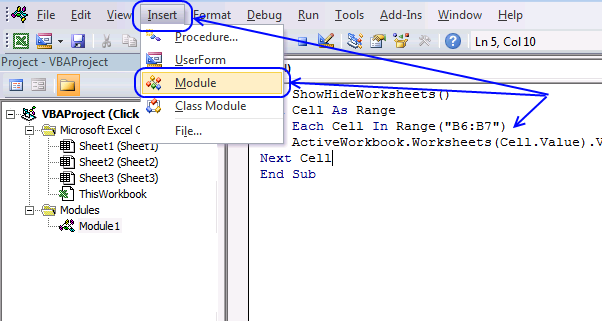
(The macro shown in the image above is not used in this article, it only shows you where to paste the code.)
- Press Alt-F11 to open the visual basic editor
- Press with left mouse button on Module on the Insert menu
- Copy and paste the above user defined function
- Exit visual basic editor
- Select a cell (B1)
- Type =Ins_text_qualifiers(A1) into formula bar and press ENTER
Text to columns (Excel 2007)
- Select "Data" tab on the ribbon
- Press with left mouse button on "Text to columns" button
10. Extract values between two given delimiting strings

The image above demonstrates a rather small formula in cell D3 that extracts values in cell B3 based on two given strings or delimiters.
10.1 Extract values between two given delimiting strings

Cell B3 contains phone numbers, they start with a given string "#" and end with another string "|". The formula is able to extract any value without any changes to the formula, this example demonstrates phone numbers.
The delimiting strings may contain multiple characters if needed. The dynamic array formula in cell D3 extracts each value between these strings and spills values below as far as needed automatically.
Excel 365 formula in cell D3:
Explaining formula
Step 1 - Create an array based on the last delimiting string
The TEXTSPLIT function splits a string into an array across columns and rows based on delimiting characters.
TEXTSPLIT(Input_Text, col_delimiter, [row_delimiter], [Ignore_Empty])
TEXTSPLIT(B3, , "|", TRUE)
becomes
TEXTSPLIT("Fake phone numbers: #555-6426262|and #555-5769326| and #555-94721| or #555-79324|", , "|", TRUE)
and returns
{"Fake phone numbers: #555-6426262"; "and #555-5769326"; " and #555-94721"; " or #555-79324"}.
Step 2 - Remove characters before the first delimiting string
The TEXTAFTER function extracts a string after a specific substring in a given value.
TEXTAFTER(input_text,text_after, [n], [ignore_case])
TEXTAFTER(TEXTSPLIT(B3,,"|",TRUE),"#",,,,"")
becomes
TEXTAFTER({"Fake phone numbers: #555-6426262"; "and #555-5769326"; " and #555-94721"; " or #555-79324"},"#",,,,"")
and returns
{"555-6426262"; "555-5769326"; "555-94721"; "555-79324"; ""}.

This formula is not much different from the one above, except that it allows you to specify delimiting strings in cells E2 and E3 respectively.
Excel 365 formula in cell D6:
There are leading and trailing spaces in the example above, use the TRIM function to remove those.
Excel 365 formula in cell D6:
10.2. Extract values between two given delimiting strings in a cell range

The following formula lets you extract values between two given strings from a cell range.
Excel 365 formula in cell D3:
TEXTJOIN function character limit
Explaining formula
Step 1 - Merge values
The TEXTJOIN function merges values from multiple cell ranges and also use delimiting characters if you want.
TEXTJOIN(delimiter, ignore_empty, text1, [text2], ...)
TEXTJOIN(, , B3:B10)
becomes
TEXTJOIN(, , {"Fake phone numbers: #555-6426262|and #555-5769326| and #555-94721| or #555-79324|";0;0;0;0;0;0;"Fake random phone numbers: #555-28462|and #555-19283| and #555-8883452| ? #555-6532877|"})
and returns
"Fake phone numbers: #555-6426262|and #555-5769326| and #555-94721| or #555-79324|Fake random phone numbers: #555-28462|and #555-19283| and #555-8883452| ? #555-6532877|".
Step 2 - Create an array based on the last delimiting string
The TEXTSPLIT function splits a string into an array across columns and rows based on delimiting characters.
TEXTSPLIT(Input_Text, col_delimiter, [row_delimiter], [Ignore_Empty])
TEXTSPLIT(TEXTJOIN(, , B3:B10), , "|", TRUE)
becomes
TEXTSPLIT("Fake phone numbers: #555-6426262|and #555-5769326| and #555-94721| or #555-79324|Fake random phone numbers: #555-28462|and #555-19283| and #555-8883452| ? #555-6532877|", , "|", TRUE)
and returns
{"Fake phone numbers: #555-6426262"; "and #555-5769326"; " and #555-94721"; " or #555-79324"; "Fake random phone numbers: #555-28462"; "and #555-19283"; " and #555-8883452"; " ? #555-6532877"}
Step 3 - Remove characters before the first delimiting string
The TEXTAFTER function extracts a string after a specific substring in a given value.
TEXTAFTER(input_text,text_after, [n], [ignore_case])
TEXTAFTER(TEXTSPLIT(TEXTJOIN(, , B3:B10), , "|", TRUE), "#")
becomes
TEXTAFTER({"Fake phone numbers: #555-6426262"; "and #555-5769326"; " and #555-94721"; " or #555-79324"; "Fake random phone numbers: #555-28462"; "and #555-19283"; " and #555-8883452"; " ? #555-6532877"}, "#")
and returns
{"555-6426262";"555-5769326";"555-94721";"555-79324";"555-28462";"555-19283";"555-8883452";"555-6532877"}
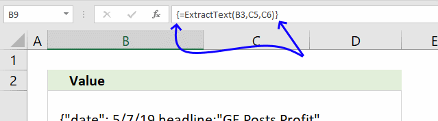
11. Extract text between words - UDF
I have a somewhat related question, if you don't mind:
I have very large amount of text in a single cell, and I would like to extract multiple instances of text that appear between two specific words.
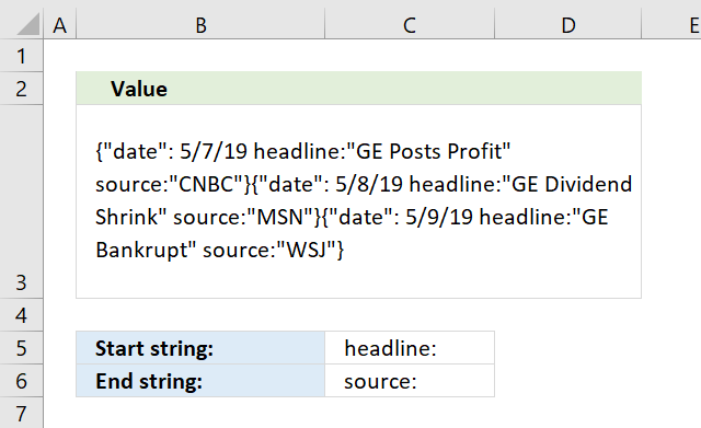
For example, here is the sample text in one cell:
{"date": 5/7/19 headline:"GE Posts Profit" source:"CNBC"}{"date": 5/8/19 headline:"GE Dividend Shrink" source:"MSN"}{"date": 5/9/19 headline:"GE Bankrupt" source:"WSJ"}
This following formula does a good enough job of extracting the first headline:
=MID(C2,SEARCH("headline",C2)+2,SEARCH("source:",C2)-SEARCH("headline",C2)-4)
However it only extracts the first headline and nothing after it.
If possible, I would like to extract all of headlines within the text in that cell, and generate a vertical array of those headlines so that it looks like this:
GE Posts Profit
GE Dividends Shrink
GE Bankrupt
Is this possible?
Thanks very much.
Update! Excel 365 users check this article: Extract values between two given delimiting strings
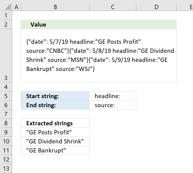
The array formula that I entered in cell range B9:B11 is a user-defined function that I created. It extracts text from cell B3 based on a start and end string specified in cell C5 and C6 respectively.
Before using it you need to copy the VBA code below and paste it to a regular code module, instructions below.
Array formula in cell range B9:B11
To enter the array formula select cell range B9:B11. Type the formula and then press and hold CTRL + SHIFT simultaneously, now press Enter once. Release all keys.
The formula bar now shows the formula with a beginning and ending curly bracket telling you that you entered the formula successfully. Don't enter the curly brackets yourself.
11.1 User Defined Function Syntax
ExtractText(text, start_word, end_word)
11.2 Arguments
| text | Required. A cell reference to the cell containing the text you want to extract. |
| start_word | Required. The first word you want to search for. |
| end_word | Required. The second word you want to search for. Text between the first and second word will be extracted, even if there are multiple instances. |
11.3 VBA code
Function ExtractText(text As String, start_word As String, end_word As String)

'Dimension variables and declare data types
Dim tmpArr() As Variant

'Count instances
ccount = UBound(Split(text, start_word)) - 1
ReDim tmpArr(ccount)


'Iterate through text string
For i = 0 To ccount

    'Find start position of instance
    StartStr = InStr(text, start_word) + Len(start_word)

    'Find end position of instance
    EndStr = InStr(text, end_word)

    'Extract first instance
    tmpArr(i) = Mid(text, StartStr, EndStr - StartStr)

    'Remove instance and save to variable again
    text = Mid(text, EndStr + Len(EndStr), Len(text))


Next i

ExtractText = Application.Transpose(tmpArr)

End Function
11.4 Where do I put the code above?
- Copy code above.
- Go to tab "Developer", press with left mouse button on the "Visual Basic" button to open VB Editor.
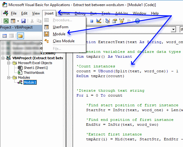
- Press with left mouse button on "Insert" on the menu.
- Press with left mouse button on "Module" to insert a module to your workbook.
- Paste code to code module, see above image.
- Exit VB Editor and return to Excel.
12. Split words in a cell range into a cell each [UDF]

This example demonstrates a user defined function (udf) that splits strings in agiven cell range to a cell each. The image above shows random values in cell range A1:A10.
Cell range C2:C27 contains an array formula, here is how to enter this udf as an array formula:
- Select all the cells to be filled, C2:C27
- Type the array formula SplitWords($A$1:$A$10) in the formula bar.
- Press and hold Ctrl + Shift simultaneously.
- Press Enter once.
- Release all keys.
The formula now looks like this: {=SplitWords($A$1:$A$10)}
Don't enter these curly brackets yourself, they appear automatically.
User defined function: Read Rick Rothstein's (MVP - Excel) comment!
'Name user defined function and declare parameters
Function SplitWords(rng As Range) As Variant()

'Dimension variables and their data types
Dim x As Variant, Wrds() As Variant, Cells_row As Long
Dim Cells_col As Long, Words As Long, y() As Variant

'Redimension variable y
ReDim y(0)

'Save values in given cell range to variable Wrds
Wrds = rng.Value

  'Iterate through rows in array variable Wrds
  For Cells_row = LBound(Wrds, 1) To UBound(Wrds, 1)

    'Iterate through columns in array variable Wrds
    For Cells_col = LBound(Wrds, 2) To UBound(Wrds, 2)

      'Split text string in given array container to a new array variable named x. The Split function returns an array of substrings based on a delimiting character and a given string .
      x = Split(Wrds(Cells_row, Cells_col))

      'Iterate through values in array variable x
      For Words = LBound(x) To UBound(x)

        'Save value to last array contain in variable y
        y(UBound(y)) = x(Words)

        'Add a new array container
        ReDim Preserve y(UBound(y) + 1)

      'Continue with the next value in array variable Words
      Next Words

    'Continue with the next column
    Next Cells_col

  'Continue with the next row
  Next Cells_row

'Rearrange (transpose) values in variable y and return those values to the worksheet.
SplitWords = Application.Transpose(y)

End Function
Where to copy the code
- Press with left mouse button on "Developer" tab on the ribbon
How to enable developer tab on the ribbon - Press with left mouse button on "Visual Basic" button
- Insert a new module
- Copy this udf example and paste it into new module
13. Split words in a cell range into a cell each - Excel 365
This formula works only in Excel 365, it extracts strings between spaces in a cell range and returns each string to a cell.
Excel 365 formula in cell C2:
Explaining formula
Step 1 - Merge cell values
Deprecated: Function get_page_by_title is deprecated since version 6.2.0! Use WP_Query instead. in /var/www/html/get-digital-help.com/public_html/wp-includes/functions.php on line 6031
The TEXTJOIN function combines text strings from multiple cell ranges.
Function syntax: TEXTJOIN(delimiter, ignore_empty, text1, [text2], ...)
TEXTJOIN(" ", TRUE, A1:A10)
becomes
TEXTJOIN(" ", TRUE, {"Cessna 150"; "Cessna 172 Skyhawk"; "Cessna T-37 Tweet"; "Piper PA-18 Super Cub"; "Piper Continental C-90-8F"; "Piper Lycoming O-320"; "Beechcraft 390"; "Beechcraft 400"; "Beechcraft 1900"; "Beechcraft 2000"})
and returns
"Cessna 150 Cessna 172 Skyhawk Cessna T-37 Tweet Piper PA-18 Super Cub Piper Continental C-90-8F Piper Lycoming O-320 Beechcraft 390 Beechcraft 400 Beechcraft 1900 Beechcraft 2000".
Step 2 - Split text based on a space character as a delimiting character
Deprecated: Function get_page_by_title is deprecated since version 6.2.0! Use WP_Query instead. in /var/www/html/get-digital-help.com/public_html/wp-includes/functions.php on line 6031
The TEXTSPLIT function splits a string into an array based on delimiting values.
Function syntax: TEXTSPLIT(Input_Text, col_delimiter, [row_delimiter], [Ignore_Empty])
TEXTSPLIT(TEXTJOIN(" ", TRUE, A1:A10),," ",TRUE)
becomes
TEXTSPLIT("Cessna 150 Cessna 172 Skyhawk Cessna T-37 Tweet Piper PA-18 Super Cub Piper Continental C-90-8F Piper Lycoming O-320 Beechcraft 390 Beechcraft 400 Beechcraft 1900 Beechcraft 2000",," ",TRUE)
and returns
{"Cessna";"150";"Cessna";"172";"Skyhawk";"Cessna";"T-37";"Tweet";"Piper";"PA-18";"Super";"Cub";"Piper";"Continental";"C-90-8F";"Piper";"Lycoming";"O-320";"Beechcraft";"390";"Beechcraft";"400";"Beechcraft";"1900";"Beechcraft";"2000"}
Split values category
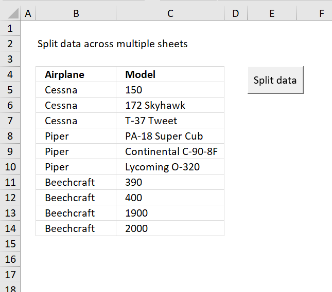
Table of Contents Split data across multiple sheets - VBA Add values to worksheets based on a condition - VBA […]
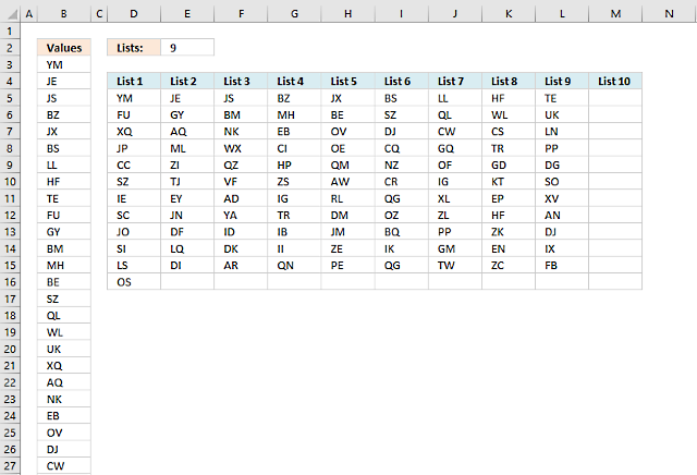
Table of Contents Split values equally into groups Rearrange values based on category - VBA 1. Split values equally […]
This article demonstrates two ways to calculate expenses evenly split across multiple people. The first one is a formula solution, […]
Excel categories
45 Responses to “A Comprehensive Guide to Splitting Text in Excel”
Leave a Reply
How to comment
How to add a formula to your comment
<code>Insert your formula here.</code>
Convert less than and larger than signs
Use html character entities instead of less than and larger than signs.
< becomes < and > becomes >
How to add VBA code to your comment
[vb 1="vbnet" language=","]
Put your VBA code here.
[/vb]
How to add a picture to your comment:
Upload picture to postimage.org or imgur
Paste image link to your comment.
You have way more lines of code in your UDF than you need. Give this UDF a try instead...
Function SplitWords(Rng As Range) As Variant
SplitWords = WorksheetFunction.Transpose(Split(Join( _
WorksheetFunction.Transpose(Rng))))
End Function
The function is actually a one-liner, but I posted it with a line continuation so that your comment processor wouldn't word-wrap it at a "funny" location.
>> SplitWords($A$1:$A$10) + CTRL + SHIFT + ENTER.
>> Copy cell C2 and paste it down as far as needed.
By the way, is the above really how you implemented your UDF? I can't get your or my version of the function to work correctly using the above procedure... I am not sure what I am missing. Instead, I select all the cells to be filled, then type the formula into the Formula Bar and press CTRL+SHIFT+ENTER... doing it that way automatically fills the selected range correctly.
Rick Rothstein (MVP - Excel),
Many thanks!!
You will probably find more lengthy code here in the future, I was planning on blog posts like "Unique distinct words from a cell range (udf)" and "Duplicate words from a cell range (udf)". But I am sure I can´t write genious code like that. I am grateful, I have learned new things today!
You are also right about how to implement the udf. Thanks for your contribution!
@Oscar,
Below is a version of the SplitWords UDF that may be more useful than either of the two UDFs that we posted earlier. The problem with our current UDFs is that if you select a larger range to put the UDF formulas in than is required for the current range being processed, you get errors displayed in the cells that do not get populated with words. There are two reasons you might want to select a larger range of cells to populate with the UDF formula... one, you don't know how many cells to select because you don't know where the end of the split word list will be; two, you want to pass a larger range to the UDF so that you can dynamically handle new rows of data in the future and you want to populate the UDF formula through enough cells to handle such a future expansion to that original list. Using your sample worksheet with its 10 rows of data, replace whatever SplitWords UDF you current have with this one...
Function SplitWords(Rng As Range) As Variant
Dim List As String, Words As Variant
Application.Volatile
With WorksheetFunction
List = .Trim(Join(.Transpose(Rng)))
Words = Split(List)
List = List & Space(Application.Caller.Count - UBound(Words))
SplitWords = .Transpose(Split(List))
End With
End Function
Now select, say, the range C2:C60 (this should be large enough to handle new words added to the list) and then put this formula in the Formula Bar...
=SplitWords(A1:A20)
and commit the formula using CTRL+SHIFT+ENTER (notice the range argument covers more cells than the number of cells with data in them... this is to be able to handle future entries in A11, A12, etc.). Okay, after you have done the above, the first thing to notice is that there are no errors being displayed in the cells that do not get populated with words. The second thing to notice is you can now fill in new data in cells A11 thru A20 and those words will get placed in the list in cells C2:C60. On top of that, if you skip rows in the word list range (that is, with your existing list of words in A1 thru A10, put "one two three" in, say, A18), the intervening blank rows will not be displayed in the resulting list of individual words in Column C. Hopefully, you and your readers will find this new version of the SplitWords UDF useful.
@Oscar,
Whoops! I left a line of code in there from previous testing that can be removed. The Application.Volatile statement is not needed (that was left over from earlier attempts to correct code that was not working correctly). The UDF you and your readers should use is this one...
Function SplitWords(Rng As Range) As Variant
Dim List As String, Words As Variant
With WorksheetFunction
List = .Trim(Join(.Transpose(Rng)))
Words = Split(List)
List = List & Space(Application.Caller.Count - UBound(Words))
SplitWords = .Transpose(Split(List))
End With
End Function
Oh, by the way... I'd like to take a crack at the "Unique distinct words from a cell range (udf)" and "Duplicate words from a cell range (udf)" code that you mentioned, but I have a question as to what you want for the final output in that first one... Is the unique distinct word list to be only those words that do not have a duplicate elsewhere in the list, or a list of all words but only listed one time (without their duplicates)? If you do not want me to post these before you had a chance to try your hand at them, just say so. If that will be the case, then you can send me your email address and I'll foward any solutions I come up with directly to you so that you can incorporate them in your future article if you wish. Let me know either way how you want me to handle this.
@Oscar,
Sigh! It seems I omitted a boundary check. My lastest UDF will produce a series of #VALUE! errors if the selected range is not large enough to house all the words in the split out list. Here is the corrected code...
Function SplitWords(Rng As Range) As Variant
Dim List As String, Words As Variant
With WorksheetFunction
List = .Trim(Join(.Transpose(Rng)))
Words = Split(List)
If Application.Caller.Count > UBound(Words) Then
List = List & Space(Application.Caller.Count - UBound(Words))
End If
SplitWords = .Transpose(Split(List))
End With
End Function
Rick Rothstein (MVP - Excel),
I would be more than happy if you would like to try to solve those problems. Actually there are three problems:
Unique - Words occurring only once.
Unique distinct - List of all words but only listed one time without their duplicates
Duplicate - Words having duplicates.
You can post or email your solutions.
Thanks for all your work!!
@Oscar,
Here are the functions I have developed. I am going to sleep now, so I have not had time to test them fully, but I am pretty sure they work. Note that there is an optional argument allowing you to specify whether the matches will be case sensitive or not... the default is False, that is, to not match case so that One, one and ONE would be considered the same... specifying True for the optional argument would mean those three words would be considered as being different. These function are array functions and should be implemented by selecting the range to be filled (you can select more cells that will be necessary so that the list will dynamically expand if more words are added) and then committed by pressing CTRL+SHIFT+ENTER. You can specify a larger range for the first argument so that additional cells can be filled with words later on. Okay, here are the functions...
Function DuplicateWords(Rng As Range, Optional _
MatchCase As Boolean) As Variant
Dim X As Long, WordCount As Long, List As String
Dim Duplicates As Variant, Words() As String
List = WorksheetFunction.Trim(Join(WorksheetFunction.Transpose(Rng)))
Words = Split(List)
For X = 0 To UBound(Words)
If MatchCase Then
If UBound(Split(" " & UCase(List) & " ", _
" " & UCase(Words(X)) & " ")) > 1 Then
Duplicates = Duplicates & StrConv(Words(X), vbProperCase) & " "
List = Replace(List, Words(X), "")
End If
Else
If UBound(Split(" " & List & " ", " " & Words(X) & " ")) > 1 Then
Duplicates = Duplicates & Words(X) & " "
List = Replace(List, Words(X), "")
End If
End If
Next
Duplicates = WorksheetFunction.Trim(Duplicates)
Words = Split(Duplicates)
If Application.Caller.Count > UBound(Words) Then
Duplicates = Duplicates & Space(Application.Caller.Count - UBound(Words))
End If
DuplicateWords = WorksheetFunction.Transpose(Split(Duplicates))
End Function
Function UniqueWords(Rng As Range, Optional MatchCase As Boolean) As Variant
Dim X As Long, WordCount As Long, List As String
Dim Uniques As Variant, Words() As String
List = WorksheetFunction.Trim(Join(WorksheetFunction.Transpose(Rng)))
Words = Split(List)
For X = 0 To UBound(Words)
If MatchCase Then
If UBound(Split(" " & UCase(List) & " ", _
" " & UCase(Words(X)) & " ")) = 1 Then
Uniques = Uniques & StrConv(Words(X), vbProperCase) & " "
List = Replace(List, Words(X), "")
End If
Else
If UBound(Split(" " & List & " ", " " & Words(X) & " ")) = 1 Then
Uniques = Uniques & Words(X) & " "
List = Replace(List, Words(X), "")
End If
End If
Next
Uniques = WorksheetFunction.Trim(Uniques)
Words = Split(Uniques)
If Application.Caller.Count > UBound(Words) Then
Uniques = Uniques & Space(Application.Caller.Count - UBound(Words))
End If
UniqueWords = WorksheetFunction.Transpose(Split(Uniques))
End Function
Function ListOfWords(Rng As Range, Optional MatchCase As Boolean) As Variant
Dim X As Long, Index As Long, List As String
Dim Words() As String, LoW As Variant
With WorksheetFunction
Words = Split(.Trim(Join(.Transpose(Rng))))
LoW = Split(Space(.Max(UBound(Words), Application.Caller.Count) + 1))
For X = 0 To UBound(Words)
If InStr(1, Chr(1) & List & Chr(1), Chr(1) & Words(X) & _
Chr(1), 1 - Abs(MatchCase)) = 0 Then
List = List & Chr(1) & Words(X)
LoW(Index) = Words(X)
Index = Index + 1
End If
Next
ListOfWords = .Transpose(LoW)
End With
End Function
@Oscar,
I think I must have been sleepier than I thought when I concocted those macros... there appear to be some minor problems with them... give me some time to investigate and straighten them out.
@Oscar,
Okay, I think I have everything straightened out now. I'll list the code in a moment; but, to make things easier, here is a link where you can get a workbook with some sample data and the all the codes already implemented (and formatted so they are more readable that the codes listed below. That link is...
https://www.filefactory.com/file/b361f7f/n/Word_Listing_Code.xls
I noticed in my previous listings that when I didn't put line continuations on lines that were long enough to word-wrap, that copying those lines from your comment processor's listing "straightened out" the word-wrapped lines; so, I have decided not to try and insert any line continuations assuming you and your readers will be copy/pasting my code into a VB editor code window. So below are my macros for your three stated needs...
Unique - Words occurring only once.
Unique distinct - List of all words but only listed one time without their duplicates.
Duplicate - Words having duplicates.
Let me know how they work out for you or (hopefully not) about any bugs you might find in them...
Function DuplicatedWords(Rng As Range, Optional CaseSensitive As Boolean) As Variant
Dim X As Long, WordCount As Long, List As String, Duplicates As Variant, Words() As String
List = WorksheetFunction.Trim(Replace(Join(WorksheetFunction.Transpose(Rng)), Chr(160), " "))
Words = Split(List)
For X = 0 To UBound(Words)
If CaseSensitive Then
If UBound(Split(" " & List & " ", " " & Words(X) & " ")) > 1 Then
Duplicates = Duplicates & Words(X) & " "
List = Replace(List, Words(X), "", 1, -1, vbBinaryCompare)
End If
Else
If UBound(Split(" " & UCase(List) & " ", " " & UCase(Words(X)) & " ")) > 1 Then
Duplicates = Duplicates & StrConv(Words(X), vbProperCase) & " "
List = Replace(List, Words(X), "", 1, -1, vbTextCompare)
End If
End If
Next
Duplicates = WorksheetFunction.Trim(Duplicates)
Words = Split(Duplicates)
If Application.Caller.Count > UBound(Words) Then
Duplicates = Duplicates & Space(Application.Caller.Count - UBound(Words))
End If
DuplicatedWords = WorksheetFunction.Transpose(Split(Duplicates))
End Function
Function UniqueWords(Rng As Range, Optional CaseSensitive As Boolean) As Variant
Dim X As Long, WordCount As Long, List As String, Uniques As Variant, Words() As String
List = WorksheetFunction.Trim(Replace(Join(WorksheetFunction.Transpose(Rng)), Chr(160), " "))
Words = Split(List)
For X = 0 To UBound(Words)
If CaseSensitive Then
If UBound(Split(" " & List & " ", " " & Words(X) & " ")) = 1 Then
Uniques = Uniques & Words(X) & " "
List = Replace(List, Words(X), "")
End If
Else
If UBound(Split(" " & UCase(List) & " ", " " & UCase(Words(X)) & " ")) = 1 Then
Uniques = Uniques & StrConv(Words(X), vbProperCase) & " "
List = Replace(List, Words(X), "")
End If
End If
Next
Uniques = WorksheetFunction.Trim(Uniques)
Words = Split(Uniques)
If Application.Caller.Count > UBound(Words) Then
Uniques = Uniques & Space(Application.Caller.Count - UBound(Words))
End If
UniqueWords = WorksheetFunction.Transpose(Split(Uniques))
End Function
Function ListOfWords(Rng As Range, Optional CaseSensitive As Boolean) As Variant
Dim X As Long, Index As Long, List As String, Words() As String, LoW As Variant
With WorksheetFunction
Words = Split(.Trim(Replace(Join(.Transpose(Rng)), Chr(160), " ")))
LoW = Split(Space(.Max(UBound(Words), Application.Caller.Count) + 1))
For X = 0 To UBound(Words)
If InStr(1, Chr(1) & List & Chr(1), Chr(1) & Words(X) & Chr(1), 1 - Abs(CaseSensitive)) = 0 Then
List = List & Chr(1) & Words(X)
If CaseSensitive Then
LoW(Index) = Words(X)
Else
LoW(Index) = StrConv(Words(X), vbProperCase)
End If
Index = Index + 1
End If
Next
ListOfWords = .Transpose(LoW)
End With
End Function
And, to keep all the code in one place, here is my last posted SplitWord macro...
Function SplitWords(Rng As Range) As Variant
Dim List As String, Words As Variant
With WorksheetFunction
List = .Trim(Replace(Join(.Transpose(Rng)), Chr(160), " "))
Words = Split(List)
If Application.Caller.Count > UBound(Words) Then
List = List & Space(Application.Caller.Count - UBound(Words))
End If
SplitWords = .Transpose(Split(List))
End With
End Function
All of these macros share the same functionality; namely, that one, you can select far more cells to load the formulas in than are required by the list (the empty text string will be displayed for cells not having an entry)... two, you can specify a larger range than the there are filled in cells as the argument to these macros to allow for future entries in the column... and three, for all but the SplitWords macro, you can specify whether the listing is to be case sensitive or not via the optional second argument with the default value being FALSE, meaning duplicated entries with different casing (like One, one, ONE, onE, etc.) will all be treated as if they were the same word with the same spelling... if you pass TRUE for that optional second argument, then those words would all be treated as if they were different words. One note... for all the "Case Insensitive" listing, the words are listed in Proper Case (first letter upper case, remaining letters lower case), the reason being if you had One, one and ONE then there is not reason to prefer one version over another, so I solve the problem by using Proper Case throughout. And, finally, as a reminder for your readers, these macros are implemented by first selecting a range to fill (remember, you can select more than will be required for you existing list in case more data is added later), then press with left mouse button on the Formula Bar and typing the UDF formula and then, finally, commiting the formula using CTRL+SHIFT+ENTER (not just Enter by itself).
Rick Rothstein (MVP - Excel),
Great work!! I will post your code, explanations and your name in future blog articles.
Now I need to understand your code.
Thanks!!
Edited: 2010-09-13 10:52
I guess your "Great work" comment meant my macros passed your testing. As for understanding the code.. please feel free to ask for any explanations you might need.
@Oscar,
First off, I just wanted to let you know your posted code got messed up at the first For statement... that line became combined with the line that follows it. Second, you have these two lines of code in your code...
If Asc(Mid(Str, i, 1)) >= 65 And Asc(Mid(Str, i, 1)) <= 90 Or _ Asc(Mid(Str, i, 1)) >= 90 And Asc(Mid(Str, i, 1)) <= 122 Then If Asc(Mid(Str, Len(Str), 1)) >= 65 And Asc(Mid(Str, _
Len(Str), 1)) <= 90 Or Asc(Mid(Str, Len(Str), 1)) >= 90 And _
Asc(Mid(Str, Len(Str), 1)) <= 122 Then Str = Str & "'" Both of the tested ranges meet at ASCII 90 meaning they can be replaced by these single range tests instead... If Asc(Mid(Str, i, 1)) >= 65 And Asc(Mid(Str, i, 1)) <= 122 Then If Asc(Mid(Str, Len(Str), 1)) >= 65 And _
Asc(Mid(Str, Len(Str), 1)) <= 122 Then Str = Str & "'" If that is really what you meant for your test range, then I wanted to point out your original two statements can be greatly simplified using the Like operator to these... If Mid(Str, i, 1) Like "[A-z]" Then If Mid(Str, Len(Str), 1) Like "[A-z]" Then Str = Str & "'" Now, I'm guessing you didn't mean the two ranges being tested to meet as the letter "Z"; rather, I think you may have simply mistyped 90 in the second range for 97 (the ASCII code for "a"). If that is the case, you will need to change your posted code and the code in your example worksheet accordingly. Oh, if you want, the Like operator can help out for this as well... If Asc(Mid(Str, i, 1)) Like "[A-Za-z]" Then If Asc(Mid(Str, Len(Str), 1)) Like "[A-Za-z]" Then Str = Str & "'"
I have made the corrections!
Thanks!!
Assuming VB code is permitted, this problem may be better handled with event code rather than formulas. With event code, you do not have to guess at how many rows or columns to copy the formula into... the code will adapt to whatever number of entries are made and for whatever number of words are in the text for those entries. Press with right mouse button on the name tab for the worksheet you want this functionality on, select View Code from the popup menu that appears and then copy paste the following code into the code window that opened up...
Private Sub Worksheet_Change(ByVal Target As Range)
  Dim Cell As Range, Words() As String
  Const WordColumn As String = "B"
  Const OutputOffset As Long = 2
  If Not Intersect(Target, Columns(WordColumn)) Is Nothing Then
    If Intersect(Target, Columns(WordColumn)) = Target Then
      For Each Cell In Target
        Words = Split(WorksheetFunction.Trim(Cell.Value))
        Range(Cells(Target.Row, WordColumn).Offset(0, _
              OutputOffset), Cells(Target.Row, _
              Columns.Count)).ClearContents
        Target.Offset(0, OutputOffset).Resize(1, _
               UBound(Words) + 1).Value = Words
      Next
    End If
  End If
End Sub
That is it... go back to the worksheet and type some words in Column B and watch the words appear in Column D outward.
Thanks for your contribution!
I tried Using the Array formula with .formulaarry in Excel, but I get 1004 error.
How do I Use the above array formula in VB ??
Sree Pavan,
Why use the array formula in vba?
I would use Rick Rothstein´s vb code instead.
Why not copy the array formula into the formula bar?
Hi Oscar,
I dont need all the texts from the column, I need only a few words\numbers & in non consecutive columns.
For Example :
Column A has "Cat Rat Mat bat"
I need Mat in column D, Cat in column E & bat in column G.
The array formula works for the above scenario, but the Private sub doesnt!! :(
Sree Pavan,
Did you copy the code into a module?
Where to copy the code
Press with right mouse button on the name tab for the worksheet you want this functionality on, select View Code from the popup menu that appears and then copy paste the code into the code window that opened up...
Hi! that's really interesting, I use this feature to do that:
https://runakay.blogspot.com/2012/01/separating-one-cell-text-in-columns.html
It's great many thanks :-)
But the separated words have an extra unnecessary space before the first character (for each one of them) probably a +1/-1 problem, could you fix?
I got over it by putting your formula in a simple MID formula, that way:
=MID(MID(" "&$B2&" ", SMALL(IF(ISERROR(SEARCH(MID(" "&$B2&" ", ROW($1:$99), 1), " ")), "", ROW($1:$99)), COLUMN(A1)), SMALL(IF(ISERROR(SEARCH(MID(" "&$B2&" ", ROW($1:$99), 1), " ")), "", ROW($1:$99)), COLUMN(A1)+1)-SMALL(IF(ISERROR(SEARCH(MID(" "&$B2&" ", ROW($1:$99), 1), " ")), "", ROW($1:$99)), COLUMN(A1))),2,100)
Evyatar,
Thanks for commenting!
You are right, it is a +1/-1 problem. I added +1 inside the formula and problem solved.
Blog post updated.
:-)
Thanks but now there is an extra " " at the end of each word,
the formula should be:
=MID(" "&$B2&" ", SMALL(IF(ISERROR(SEARCH(MID(" "&$B2&" ", ROW($1:$99), 1), " ")), "", ROW($1:$99)+1), COLUMN(A1)), SMALL(IF(ISERROR(SEARCH(MID(" "&$B2&" ", ROW($1:$99), 1), " ")), "", ROW($1:$99)), COLUMN(A1)+1)-SMALL(IF(ISERROR(SEARCH(MID(" "&$B2&" ", ROW($1:$99), 1), " ")), "", ROW($1:$99)), COLUMN(A1))-1)
and again many thanks for this genius formula I was looking quit long for something like that.
Do you think of a way that I can use it on a rows formula so I'll would have to use an array formula on your array formula.
For example if I have a list of sentences and I want to check if a certain word appears in one of them?
This is now built in to 2010. Under data text to columns. This also lets you use not only spaces but other text (mine was seperatoed by ":")
Evyatar,
Thanks!!
Use countif: countif(A1:A10, "*"&B1&"*")
I think you'll find this post interesting:
https://198.74.52.105/2010/11/22/return-multiple-matches-with-wildcard-vlookup-in-excel/
joe,
Yes, "Text to columns" also exists in previous versions. I just wanted to show it is possible using array formulas.
Back when this article was first posted, I gave you a VB solution. I just came across this article again and now, although kind of late, I have a short, normally entered formula for you to consider...
=TRIM(MID(SUBSTITUTE($B2," ",REPT(" ",999)),COLUMN(A1)*999-998,999))
Put the above formula in D2 and copy it across more columns than you think you will ever need (do not worry if there is no data to fill the excess cells), then copy that row of formulas down for as many rows as you want (you do not have to stop when your data ends either since, like for the excess columns, the excess rows will simply display the empty text string ("").
Actually, given that non of your words will ever be longer than 99 characters, use this formula as it can handle many more split apart words than the version I posted earlier...
=TRIM(MID(SUBSTITUTE($B2," ",REPT(" ",99)),COLUMN(A1)*99-98,99))
Rick Rothstein (MVP - Excel),
Great formula! What an inprovement,your formula is incredibly small, simple and probably a lot faster than mine.
Thanks, I'm glad you like the formula. For those who might be interested, here is a mini-blog article of mine where I discuss the generalized format underlying this formula...
https://www.excelfox.com/forum/f22/get-field-delimited-text-string-333/
How would this formula be modified if a comma is used as a separator between text fields?
Give this version of the formula I posted in the Comments a try...
=TRIM(MID(SUBSTITUTE($A1,",",REPT(" ",99)),COLUMN(A1)*99-98,99))
If you look at the sub-thread immediately above your message in the Comments, you will find a link by me which would take you to a mini-blog article of mine that will give you the generized version of this formula so that you can modify it in anyway that you want.
[…] This should help. You will need to make some modifications though. Text to columns: Split words in a cell (excel array formula) | Get Digital Help - Microsoft Excel re… […]
I was curious if you ever thought of changing the structure
of your website? Its very well written; I love what youve got to
say. But maybe you could a little more in the way of content so people could
connect with it better. Youve got an awful lot of text for only
having 1 or two pictures. Maybe you could space it out better?
There is some problem to use this formula
There is no numeric value when I used it ( there are words only)
Some time this way is breaking the words (like "Bank" breaked into "Ba nk" ) into 2 or more cells
Which should not be broken
Anil,
Which formula are you using?
=TRIM(MID(SUBSTITUTE($A1,",",REPT(" ",99)),COLUMN(A1)*99-98,99))
This one
And one thing more it is seperating in column way (means from left to right)
I want "up to down way" in only one row
Is there any way or formula?
Anil,
Can you provide a value that returns an error?
Dear Oscar,
I am facing problem with the formula when I want to start this from column number AD & row 1. Below have attached my formula which I used in my excel.
=MID(" "&$AD2&" ",SMALL(IF(ISERROR(SEARCH(MID(" "&$AD2&" ",ROW($1:$99),1)," ")),"",ROW($1:$99)+1),COLUMN(AC1)),SMALL(IF(ISERROR(SEARCH(MID(" "&$AD2&" ",ROW($1:$99),1)," ")),"",ROW($1:$99)),COLUMN(AC1)+1)-SMALL(IF(ISERROR(SEARCH(MID(" "&$AD2&" ",ROW($1:$99),1)," ")),"",ROW($1:$99)),COLUMN(AC1))-1)
AC AD AE AF AG
car 123 A #NUM!
boat 234 AD T
airplane 345 A
bus 456 AV
train 567 A V
Dipankar
What is the problem?
Which column contains your data?
I get an error when I use this code. I followed everything to a T...
"Invalid Name Error"
Bob,
which vba row was highlighted?
Thanks for the formula. Can you please tell me what is the purpose of column(A1) in the formula? This formula is beyond my current skill level, but I want to understand it badly.
Can you tell me what is the purpose of the column A1 in the array formula?
Nice job, indeed. Thank you for sharing.