Working with COMBO BOXES [Form Controls]
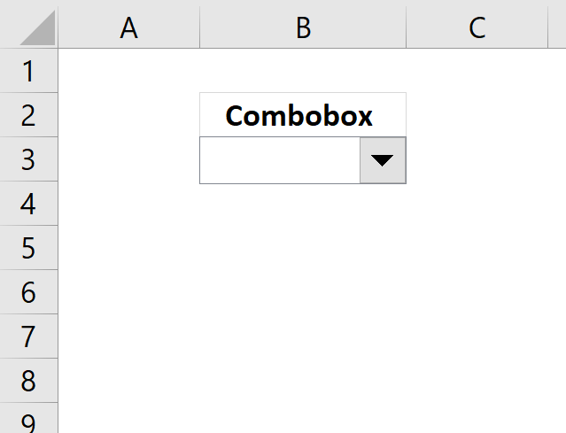
This blog post demonstrates how to create, populate and change comboboxes (form control) programmatically.
Form controls are not as flexible as ActiveX controls but are compatible with earlier versions of Excel. You can find the controls on the developer tab.
Table of Contents
- Create a combo box using vba
- Assign a macro - Change event
- Add values to a combo box
- Remove values from a combo box
- Set the default value in a combo box
- Read selected value
- Link selected value
- Change combo box properties
- Populate combo box with values from a dynamic named range
- Populate combo box with values from a table
- Currently selected combobox
- Populate a combo box (form control)
- Populate a combo box with values from a pivot table - VBA
- Apply dependent combo box selections to a filter
Watch this video about Combo Boxes
1. Create a combobox using vba
Sub CreateFormControl()
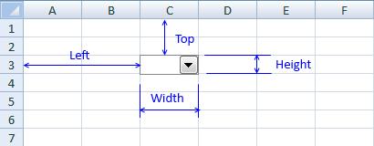
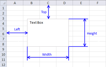
'Worksheets("Sheet1").DropDowns.Add(Left, Top, Width, Height)
Worksheets("Sheet1").DropDowns.Add(0, 0, 100, 15).Name = "Combo Box 1"
End Sub
Recommended article
Recommended articles
In this post I am going to demonstrate two things: How to populate a combobox based on column headers from […]
2. Assign a macro - Change event
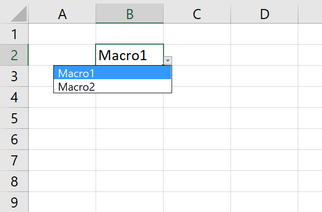
You can assign a macro to a combobox by press with right mouse button oning on the combobox and select "Assign Macro". Select a macro in the list and press ok!

This subroutine does the same thing, it assigns a macro named "Macro1" to "Combo box 1" on sheet 1. Macro1 is rund as soon as the selected value in the combo box is changed.
Sub AssignMacro()
Worksheets("Sheet1").Shapes("Combo Box 1").OnAction = "Macro1"
End Sub
Recommended article
Recommended articles
This article demonstrates how to run a VBA macro using a Drop Down list. The Drop Down list contains two […]
3. Add values to a combo box
You can add an array of values to a combo box. The list method sets the text entries in a combo box, as an array of strings.

Sub PopulateCombobox1()
Worksheets("Sheet1").Shapes("Combo Box 1").ControlFormat.List = _
Worksheets("Sheet1").Range("E1:E3").Value
End Sub
The difference with the ListFillRange property is that the combo box is automatically updated as soon as a value changes in the assigned range. You don´t need to use events or named ranges to automatically refresh the combo box, except if the cell range also changes in size.
Sub PopulateCombobox2()
Worksheets("Sheet1").Shapes("Combo Box 1").ControlFormat.ListFillRange = _
"A1:A3"
End Sub
You can also add values one by one.
Sub PopulateCombobox3()
With Worksheets("Sheet1").Shapes("Combo Box 1").ControlFormat
.AddItem "Sun"
.AddItem "Moon"
.AddItem "Stars"
End Sub
Recommended article
Recommended articles
A drop-down list in Excel prevents a user from entering an invalid value in a cell. Entering a value that […]
4. Remove values from a combo box
RemoveAllItems is self-explanatory.
Sub RemoveAllItems()

Worksheets("Sheet1").Shapes("Combo Box 1").ControlFormat.RemoveAllItems

End Sub
The RemoveItem method removes a value using a index number.
Sub RemoveItem()

Worksheets("Sheet1").Shapes("Combo Box 1").ControlFormat.RemoveItem 1

End Sub
The first value in the array is removed.
Recommended article
Recommended articles
A dialog box is an excellent alternative to a userform, they are built-in to VBA and can save you time […]
5. Set the default value in a combo box
The ListIndex property sets the currently selected item using an index number. ListIndex = 1 sets the first value in the array.

Sub ChangeSelectedValue()
With Worksheets("Sheet1").Shapes("Combo Box 1")
.List = Array("Apples", "Androids", "Windows")
.ListIndex = 1
End With
End Sub
Recommended article
Recommended articles
In this tutorial I am going to explain how to: Create a combo box (form control) Filter unique values and […]
6. Read selected value
The ListIndex property can also return the index number of the currently selected item. The list method can also return a value from an array of values, in a combo box. List and Listindex combined returns the selected value.

Sub SelectedValue()
With Worksheets("Sheet1").Shapes("Combo Box 1").ControlFormat
MsgBox "ListIndex: " & .ListIndex & vbnewline & "List value:" .List(.ListIndex)
End With
End Sub
Recommended article
Recommended articles
What is a Text Box? A Text Box (Form Control) in Excel is an interactive element that allows users to […]
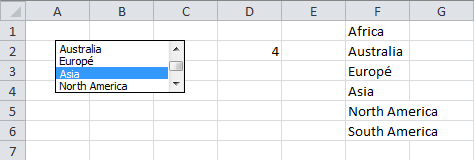
7. Link selected value
Cell F1 returns the index number of the selected value in combo box 1.

Sub LinkCell()

Worksheets("Sheet1").Shapes("Combo Box 1").ControlFormat.LinkedCell = "F1"

End Sub
Cell G1 returns the selected value in combo box 1.
Sub LinkCell2()

With Worksheets("Sheet1").Shapes("Combo Box 1").ControlFormat
    Worksheets("Sheet1").Range("G1").Value = .List(.ListIndex)
End With

End Sub
Recommended article
Recommended articles
What is a Text Box? A Text Box (Form Control) in Excel is an interactive element that allows users to […]
8. Change combobox properties
Change the number of combo box drop down lines.

Sub ChangeProperties()
Worksheets("Sheet1").Shapes("Combo Box 1").ControlFormat.DropDownLines = 2
End Sub
9. Populate combox with values from a dynamic named range

I created a dynamic named range Rng, the above picture shows how.
Sub PopulateFromDynamicNamedRange()

Worksheets("Sheet1").Shapes("Combo Box 1").ControlFormat.ListFillRange = "Rng"

End Sub
You can do the same thing as the subroutine accomplishes by press with right mouse button oning the combo box and then press with left mouse button on "Format Control...". Input Range: Rng
Back to top
10. Populate combox with values from a table

Sub PopulateFromTable()

Worksheets("Sheet1").Shapes("Combo Box 1").ControlFormat.List = _
[Table1[DESC]]

End Sub
11. Currently selected combobox
It is quite useful to know which combo box the user is currently working with. The subroutine below is assigned to Combo Box 1 and is rund when a value is selected. Application.Caller returns the name of the current combo box.
Sub CurrentCombo()

MsgBox Application.Caller

End Sub

12. Populate a combo box (form control)
In this tutorial I am going to explain how to:
- Create a combo box (form control)
- Filter unique values and populate a combo box (form control)
- Copy selected combo box value to a cell
- Refresh combo box using change events
12.1 Create a combo box (form control)

- Press with left mouse button on Developer tab on the ribbon. How to show developer tab
- Press with left mouse button on Insert button.
- Press with left mouse button on Combo box
- Create a combo box on a sheet.
(Press and hold left mouse button on a sheet. Drag down and right. Release left mouse button.)
The question now is how do you know the name of a combo box? You have to know the name when you are writing the vba code. Press with left mouse button on a combo box and the name appears in the name box.

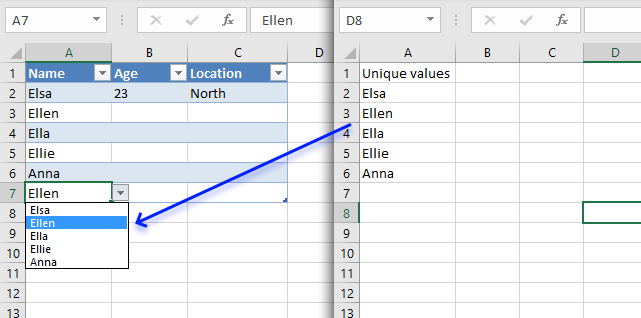
12.2 Filter unique values and populate a combo box (form control)
The code below extracts unique distinct values from column A, except cell A1. Then the code adds the extracted unique distinct values to the combo box.
'Name macro
Sub FilterUniqueData()

'Declare variables and data types
Dim Lrow As Long, test As New Collection
Dim Value As Variant, temp() As Variant

'Redimension array variable temp in order to let it grow when needed
ReDim temp(0)

'Ignore errors
On Error Resume Next

'Find last not empty cell in column A
With Worksheets("Sheet1")
  Lrow = .Range("A" & Rows.Count).End(xlUp).Row

  'Populate array temp with values from column A
  temp = .Range("A2:A" & Lrow).Value
End With

'Iterate through values in array variable temp
For Each Value In temp

   'Add value if character length is larger than 0 to test
    If Len(Value) > 0 Then test.Add Value, CStr(Value)

'Continue with next value
Next Value

'Delete all items in Combobox Drop Down 1 in sheet1
Worksheets("Sheet1").Shapes("Drop Down 1").ControlFormat.RemoveAllItems

'Populate combobox with values from test one by one
For Each Value In test
   Worksheets("Sheet1").Shapes("Drop Down 1").ControlFormat.AddItem Value
Next Value

'Clear variable
Set test = Nothing
End Sub
Copy the code into a standard module.
12.3 Copy selected combo box value to a cell
You can assign a macro to a combobox. Press with right mouse button on combobox and press with left mouse button on "Assign Macro...". See picture below.
This means when you press with left mouse button on the combobox the selected macro is run.

The vba code below copies the selected value to cell C5 whenever the combobox is selected.
- Copy the code into a standard module.
- Assign this macro to the combobox .
Sub SelectedValue()
With Worksheets("Sheet1").Shapes("Drop Down 1").ControlFormat
   Worksheets("Sheet1").Range("C5") = .List(.Value)
End With
End Sub
12.4 Refresh combo box using change events
The next step is to make the combo box dynamic. When values are added/edited or removed from column A, the combo box is instantly refreshed. Copy code below Press Alt + F11 Double press with left mouse button on sheet1 in project explorer Paste code into code window
Private Sub Worksheet_Change(ByVal Target As Range)
If Not Intersect(Target, Range("$A:$A")) Is Nothing Then
   Call FilterUniqueData
End If
End Sub

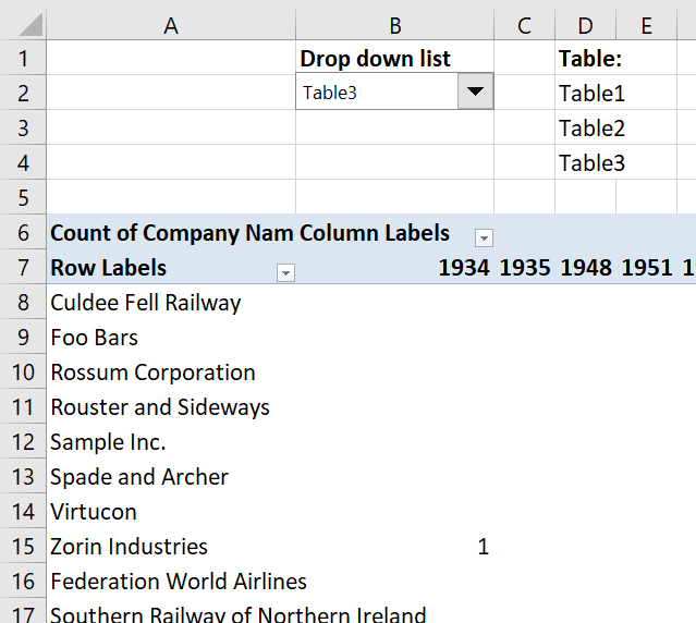
13. Populate a combobox with values from a pivot table - VBA
In this post I am going to demonstrate two things:
- How to populate a combobox based on column headers from an Excel defined Table
- Populate a combobox with unique values using a PivotTable
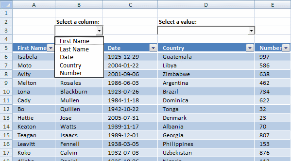
13.1 Populate a combobox with table headers
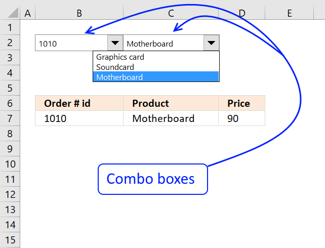
In the picture below you can see a table and two combo boxes. The table has about 50 000 rows.
Let's populate the combo box to the left with table headers, see image above.
'Name macro
Sub FillCombo1()

'Declare variables and data types
Dim Cell As Range
Dim i As Single
Dim shpobj As Object

'Assign Table1 to object Cell
Set Cell = Worksheets("Sheet1").Range("Table1")

'Clear values in ComboBox1
Worksheets("Sheet1").ComboBox1.Clear

'Go through each column in object Cell (Table1)
For i = 1 To Cell.ListObject.Range.Columns.Count

    'Add column header value to combobox
    Worksheets("Sheet1").ComboBox1.AddItem Cell.ListObject.Range.Cells(1, i)

'Continue with next column
Next i

End Sub
13.2 Populate a combo box with unique values using a Pivot Table
The selected value in the combobox to the left determines which column is going to be filtered in the PivotTable.
The combobox to the right is populated when the pivottable has processed all values. I think you get the idea when you see the picture below.

'Name macro
Sub FillCombo2()

'Declare variables and data types
Dim i As Single, r As Single
Dim shpobj As Object
Dim rng As Variant, Value As Variant

'Don't show changes
Application.ScreenUpdating = False

'Refresh PivotTable
Worksheets("Sheet2").PivotTables("PivotTable1").PivotCache.Refresh

'Ignore errors
On Error Resume Next

'Hide all fields in PivotTable
For Each ptfl In Worksheets("Sheet2").PivotTables("PivotTable1").PivotFields
    ptfl.Orientation = xlHidden
Next ptfl

'Don't ignore errrors
On Error GoTo 0

'Go through all OLEObjects (ActiveX) in Sheet1
For Each shpobj In Worksheets("Sheet1").OLEObjects

    'Find ComboBox1 and make sure it is not empty if so exit For ... Next statement
    If shpobj.Name = "ComboBox1" And shpobj.Object.Value = "" Then Exit For

    'Use the value in ComboBox1 to extract unique distinct values in PivotTable
    If shpobj.Name = "ComboBox1" Then
        Worksheets("Sheet2").PivotTables("PivotTable1") _
        .PivotFields(shpobj.Object.Value).Orientation = xlRowField
        Worksheets("Sheet2").Select

        'Make sure that the Pivot table is recalculated
        Application.Calculate
    End If

    'Check if shpobj is Combobox2
    If shpobj.Name = "ComboBox2" Then

        'Clear comboobox values
        shpobj.Object.Clear

        'Populate ComboBox2 with values from PivotTable
        shpobj.Object.List = Worksheets("Sheet2").PivotTables("PivotTable1").RowRange.Value
        shpobj.Object.RemoveItem 0
        shpobj.Object.RemoveItem _
        Worksheets("Sheet2").PivotTables("PivotTable1").RowRange.Rows.Count - 2
    End If
Next shpobj

'Activate Sheet1
Worksheets("Sheet1").Select

'Show changes for the user
Application.ScreenUpdating = True

End Sub
The pivot table is located on sheet2. Sheet1 module also contains some code:
Private Sub ComboBox1_Change()

Call FillCombo2

End Sub
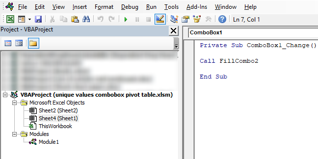
13.3 How to add code to sheet module
- Go to VB Editor (Alt + F11)
- Double press with left mouse button on Sheet4 (Sheet1) in Project Explorer, see image above. This is the sheet where ComboBox1 is located.
- Paste code to code module.
14. Apply dependent combo box selections to a filter
now if i only knew how to apply these dependent dropdown selections to a filter, i'd be set.
Answer:
Table of contents
- Overview
- Create auto expanding named ranges
- Array Formula on Calculation sheet
- Create another two auto expanding named ranges on sheet "Calculation"
- Create Combo boxes
- Setup Combo boxes
- Array Formula on Filter sheet
- Get example workbook
14.1. Overview
Filter or an excel table can accomplish this task within milliseconds but several people have asked how to do this using drop down lists.
So in this post I am going to use dependent combo-boxes instead of drop down lists.We are not going to use any vba code but we need to create a "calculation" sheet.
Why use combo box? If you decide to change a value in a combo box, other dependent combo box values change instantly. This is not the case with drop down lists.
We are going to create two combo boxes. The first combo box contains unique distinct values from column A. The second combo box contains unique distinct values from column B, based on selected value in the first combo box. See pictures below.
The data we are working with:

The final result:

If you want to create drop down lists read this article: Create dependent drop down lists containing unique distinct values in excel and then continue reading this article.
What is a unique distinct list? Remove all duplicates in a list and you have create a unique distinct list.
I have created three sheets.
- Filter
- Data
- Calculation
14.2.Create auto expanding named ranges
We are going to create two named ranges, auto expanding when new values are added. The two named ranges exists on sheet "Data"
Named range "order"
- Press with left mouse button on "Formulas" tab
- Press with left mouse button on "Name Manager"
- Press with left mouse button on "New..."
- Type a name. I named it "order". (See attached file at the end of this post)
- Type =OFFSET(Data!$A$3, 0, 0, COUNTA(Data!$A$3:$A$1000)) in "Refers to:" field.
- Press with left mouse button on "Close" button
Named range "product"
- Press with left mouse button on "Formulas" tab
- Press with left mouse button on "Name Manager"
- Press with left mouse button on "New..."
- Type a name. I named it "product". (See attached file at the end of this post)
- Type =OFFSET(Data!$B$3, 0, 0, COUNTA(Data!$B$3:$B$1000)) in "Refers to:" field.
- Press with left mouse button on "Close" button

14.3. Array Formula on sheet "Calculation"

Array formula in cell A2:
Press CTRL + SHIFT + ENTER. Copy cell A2 and paste it down as far as needed.
Array formula in cell B2:
Press CTRL + SHIFT + ENTER. Copy cell B2 and paste it down as far as needed.
The values in column B change depending on selected value in the combo box on sheet "Filter". Don´t worry, we are soon going to create the combo boxes.
14.4. Create another two auto expanding named ranges on sheet "Calculation"
The named ranges auto expands when lists change in column A and B.
Named range "uniqueorder"
- Press with left mouse button on "Formulas" tab
- Press with left mouse button on "Name Manager"
- Press with left mouse button on "New..."
- Type a name. I named it "uniqueorder". (See attached file at the end of this post)
- Type =OFFSET(Calculation!$A$2, 0, 0, COUNT(IF(Calculation!$A$2:$A$1000="", "", 1)), 1) in "Refers to:" field.
- Press with left mouse button on "Close" button
Named range "uniqueproduct"
- Press with left mouse button on "Formulas" tab
- Press with left mouse button on "Name Manager"
- Press with left mouse button on "New..."
- Type a name. I named it "uniqueproduct". (See attached file at the end of this post)
- Type =OFFSET(Calculation!$B$2, 0, 0, COUNT(IF(Calculation!$B$2:$B$1000="", "", 1)), 1) in "Refers to:" field.
- Press with left mouse button on "Close" button

14.5. Create Combo boxes
- Press with left mouse button on "Developer" tab on the ribbon
- Press with left mouse button on "Insert" button
- Press with left mouse button on Combo box button
- Place combo box on cell B2 on sheet "Filter

Create a second combo box on cell C2.

14.5.1 Setup Combo box 1
- Select sheet "Filter"
- Press with right mouse button on on combo box on cell B2
- Press with left mouse button on "Format Control..."
- Press with left mouse button on tab "Control"
- Type uniqueorder in Input range:
- Select cell B1 in Cell link:
- Press with left mouse button on OK
Setup Combo box 2
- Select sheet "Filter"
- Press with right mouse button on on combo box on cell C2
- Press with left mouse button on "Format Control..."
- Press with left mouse button on tab "Control"
- Type uniqueproduct in Input range:
- Select cell C1 in Cell link:
- Press with left mouse button on OK

I have hidden the values in cell B1 and C1.
- Select B1:C1
- Press Ctrl + 1
- Press with left mouse button on "Custom" in Category window
- Type ,,, in the "Type:" field
- Press with left mouse button on OK
14.6. Array Formula on "Filter" sheet

Array formula in cell B7:
Press CTRL + SHIFT + ENTER. Copy cell B7 and paste it to the right to cell B9. Copy cell range B7:B9 and paste it down as far as needed.
COMBO BOXES [Form Controls] examples
Check boxes in Excel are a great way to make your spreadsheets more interactive. They can be used for task […]
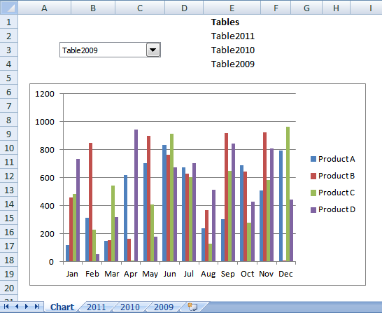
In this article I will demonstrate how to quickly change chart data range utilizing a combobox (drop-down list). The above […]
In this article, I am going to show you how to quickly change Pivot Table data source using a drop-down […]
Rahul asks: I want to know how to create a vlookup sheet, and when we enter a name in a […]
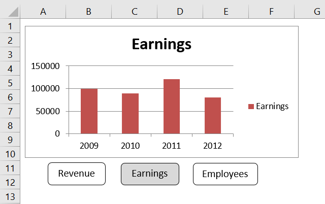
Table of Contents How to create an interactive Excel chart How to filter chart data How to build an interactive […]
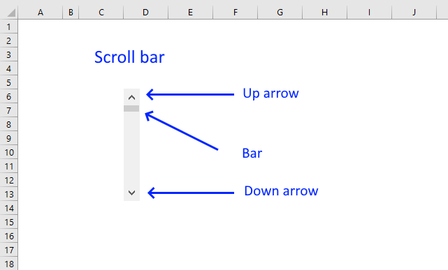
This article demonstrates how to insert and use a scroll bar (Form Control) in Excel. It allows the user to […]
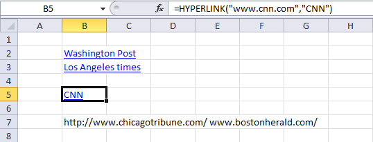
Table of Contents List all hyperlinks in worksheet programmatically Find cells containing formulas with literal (hardcoded) values Extract cell references […]
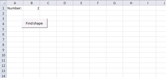
This article demonstrates how to locate a shape in Excel programmatically based on the value stored in the shape. The […]
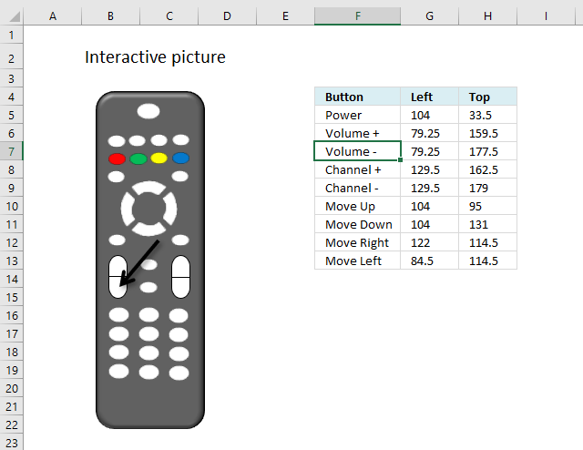
This article demonstrates how to move a shape, a black arrow in this case, however, you can use whatever shape […]
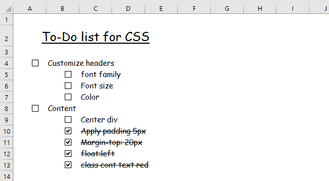
Today I will share a To-do list excel template with you. You can add text to the sheet and an […]
In this tutorial I am going to explain how to: Create a combo box (form control) Filter unique values and […]
Excel defined Tables, introduced in Excel 2007, sort, filter and organize data any way you like. You can also format […]
This article demonstrates how to run a VBA macro using a Drop Down list. The Drop Down list contains two […]
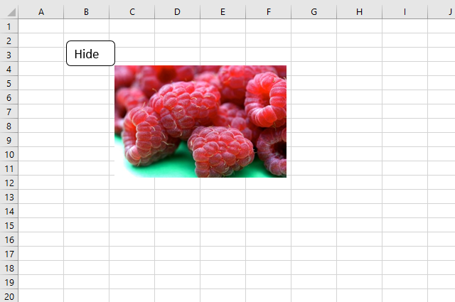
This article explains how to hide a specific image in Excel using a shape as a button. If the user […]
This article demonstrates how the user can run a macro by press with left mouse button oning on a button, […]
This blog post demonstrates how to create, populate and change comboboxes (form control) programmatically. Form controls are not as flexible […]
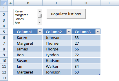
This blog post shows you how to manipulate List Boxes (form controls) manually and with VBA code. Table of Contents […]
What is a Text Box? A Text Box (Form Control) in Excel is an interactive element that allows users to […]
Combobox category
Form controls category
This article describes how to create a button and place it on an Excel worksheet, then assign a macro to […]
This blog post shows you how to manipulate List Boxes (form controls) manually and with VBA code. Table of Contents […]
What is a Text Box? A Text Box (Form Control) in Excel is an interactive element that allows users to […]
Macro category
Table of Contents How to create an interactive Excel chart How to filter chart data How to build an interactive […]
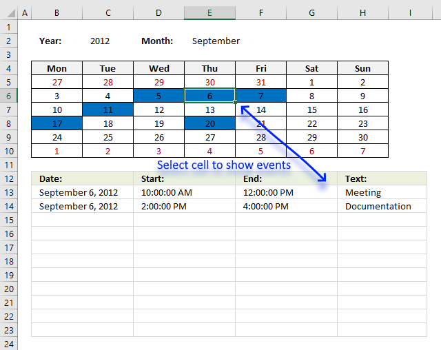
Table of Contents Excel monthly calendar - VBA Calendar Drop down lists Headers Calculating dates (formula) Conditional formatting Today Dates […]
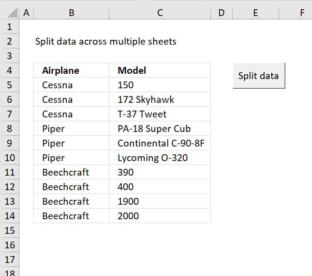
Table of Contents Split data across multiple sheets - VBA Add values to worksheets based on a condition - VBA […]
Vba category
Today I'll show you how to search all Excel workbooks with file extensions xls, xlsx and xlsm in a given folder for a […]
Table of Contents How to create an interactive Excel chart How to filter chart data How to build an interactive […]
Table of Contents Excel monthly calendar - VBA Calendar Drop down lists Headers Calculating dates (formula) Conditional formatting Today Dates […]
Excel categories
46 Responses to “Working with COMBO BOXES [Form Controls]”
Leave a Reply
How to comment
How to add a formula to your comment
<code>Insert your formula here.</code>
Convert less than and larger than signs
Use html character entities instead of less than and larger than signs.
< becomes < and > becomes >
How to add VBA code to your comment
[vb 1="vbnet" language=","]
Put your VBA code here.
[/vb]
How to add a picture to your comment:
Upload picture to postimage.org or imgur
Paste image link to your comment.
The zip file has a buch of files but non is excel 2007 .xlsm. Please repost. Thanks.
John Tseng,
That is weird.
I opened the file unique-values-combobox-pivot-table.xlsm and it is an excel 2007 macroenabled file *.xlsm.
There are no zip files in this post?
Great Article!....... I noticed that your articles are getting truncated in my Reader. Previously I used to get the complete blog directly into my reader..... Thanks again Oscar!
Your Sharing is enjoyful to me, i got some help from your posting.
precisely what I was looking for. very well done.
obie,
Thank you for commenting!
Thanks good sample.
Hello,
Very helpfull post. How can I add unique and ordered values to the combobox?
Thank you
Anibal
Anibal,
See attached file:
Populate-combo-box-unique-sorted-values.xlsm
[...] Could you please nudge me towards right direction? Thanks Rajesh have a look at sample code here Excel vba: Populate a combo box (form control) | Get Digital Help - Microsoft Excel resource You can amend code if using an active x control on your worksheet. [...]
Hi Oscar,
Thaks for the code, it works great. Could you add a third dependent combo box to this? i.e. select search type(country)/ select value (specific country)/select last name
Many thanks
Adam
Is there anyway to populate a combo box with a shape in the drop down instead of text?
Sonya,
As far as I know, no!
Excellent tutorial . . .!! simple, clear and usefull
Is there anyway to populate a combobox (ActiveX Control type) with multiple columns from a Access (2010)database table?
The file transfer does not work. Neither box get filled.
The only thing I've tried is to delete the existing selection of "Country" from combobox1 and I immediately get error 1004, unable to get pivot field properties.
I then switched to the pivot table and it was gone. ??
Any suggestions?
Allan,
run FillCombo1 macro
1. Go to tab "Developer"
2. Press with left mouse button on "Macros" button
3. Select FillCombo1
4. Press with left mouse button on the "Run" button
Now the first combobox is filled. Select a value and the second combobox is filled.
Oscar-M,
Is there anyway to populate a combobox (ActiveX Control type) with multiple columns from a Access (2010)database table?
I don´t know, try an Access forum.
Hi I tried your code, but instead of having a combo box in sheet 1, i used it in sheet2 everything is correct except if there were updates made on the selection on sheet1 the combobox in sheet2 is not updating, can you help me on this may be i miss some code?
Ver,
Try this:
Sub FilterUniqueData() Dim Lrow As Long, test As New Collection Dim Value As Variant, temp() As Variant ReDim temp(0) On Error Resume Next With Worksheets("Sheet1") Lrow = .Range("A" & Rows.Count).End(xlUp).Row temp = .Range("A2:A" & Lrow).Value End With For Each Value In temp If Len(Value) > 0 Then test.Add Value, CStr(Value) Next Value Worksheets("Sheet2").Shapes("Drop Down 1").ControlFormat.RemoveAllItems For Each Value In test Worksheets("Sheet2").Shapes("Drop Down 1").ControlFormat.AddItem Value Next Value Set test = Nothing End SubI can give a file when I get it xml file
Many thanks
[...] I wonder whether someone may be able to help me please. I'm using this example Excel vba: Populate a combo box (form control) | Get Digital Help - Microsoft Excel resource to create a combo box which contains unique values from a given spreadsheet list. If I use the [...]
could you make this macro to work on excel 2003, thanx.
[…] Hello See if this page is useful: Working with combo boxes (Form Control) using vba | Get Digital Help - Microsoft Excel resource […]
If you are going for finest contents like me, just pay a quick visit this web site everyday as it provides quality contents,
thanks
Excelente codigo. Me fue de mucha utilidad!
JULIAN LOZANO,
Gracias
[…] future issues. If you choose this approach, see quick reference on the VBA excel-form-combobox at: Working with combo boxes (Form Control) using vba | Get Digital Help - Microsoft Excel resource Good luck. Martin […]
Hello, Is there anyway to activate a form control combobox to force an user to choice an item ?
Thanks
Fanch,
Are you talking about a default value? If that is the case, check out:
Set the default value in a combo box
No default value, the user must to be notified to choive a value, the design must expand the list .
is there any way to have more spaces between the values shown in drop down list??
yes create data validation .. select from list .. create a list and write data in alternating column in list
Do you know if it is possible to select multiple items within a combobox list? Similar to Table filter options or by using Ctrl?
Wally
Do you know if it is possible to select multiple items within a combobox list?
No, you need to use a listbox (form control) or a combo box (active x).
Good Tutorial...
this is what I'm looking for
thanks
metha
thanks!
Hi Oscar,
This is very useful and thanks for this post. I need a help here:
I have a range of cells holding values for Emp name, salary, age. Same empname can have multiple rows.
I have a combobox which lists down only unique values (say Emp name) in the dropdown.
I also have a listbox which displays the row of the value selected in the combo box. While doing so, only one row is displayed when the name selected has multiple entries. Could you please help here
Can i ask: Combobox embedded in range a1:a100 with same dropdown list values. Now when user makes selection the selected text goes respectively to selected combobox reference cell. Eg ComboboxA1 txt value goes to cell A1. And same thing with the rest from A2 to A100.
So here's my dilemma: We have an Excel spreadsheet request form that users complete to make requests. One of the columns is currently a drop-down list of vendors that is from a named field. It allows them to pick the vendor on the list they want to purchase from. There are 2000-plus vendors on this list. People say it is taking too long to find their vendor on the list and they want to be able to type in a few letters to select their vendor. I got this working pretty slick with a combo box but my boss says this will make the form too large - that the combo boxes will take too much space. He wants me to use VB code instead, no combo box, to accomplish the same thing. Part of the problem I have is that we have some vendors who have multiple listings on the list - different divisions of the same vendor. They all start with the same first few letters. Without a list, I don't know how they will see the rest of the names so they can pick the right one. Suggestions? I still say the combo box is the way to go.
Hi Oscar - Is is possible to populate the dropdown from a range on another sheet?
The article was really useful
Really well written article, SIMPLE, direct to the focus.
Thanks to people like you!
Dim AppCaller As String
AppCaller = Application.Caller
MsgBox AppCaller
Getting Run time error "13" Type Mismatch on AppCaller statement. Trying to get the name of the active combo box name. Excel v16 windows 10 home.
two combobox are filled but pivot table is not correct in next sheet(sheet2)
Hi Oscar,
I was wondering if you can help me out in printing of UserForms. I have a designed a UserForm where all the data has to be entered using UserForm and recorded in one Excel Sheet. And then print out that UserForm in A4 sized paper. I have been trying by all means by as of now, I could not do so. Any kind of help would be appreciated.
I have quite a weird situation with comboboxes. I have 2 comboboxes. 1 combobox takes its items from a range (lets say F2:F20. this combobox checks the length of the data and includes it all). Based on the value selected in the other combobox the data changes in the range mentioned above.
My code seeems to work and everything seems fine. However on random occasions, when flipping back and forth between items in the combobox that changes the data that then feeds into the other combobox, i see that the data is infact incorrect and is of the previous selection. Is this because the combobox is working faster than the info is updating on the excel spreadsheet?
I can find no solution any ideas would help