How to use Excel Tables
An Excel Table is a very useful feature in Excel, it was introduced in Excel 2007. Earlier versions had this feature as well but it was then known as Excel Lists.
What can an Excel Table do for you? It will simplify your work with data, adding or removing data, filtering, totals, sorting, enhance readability using cell formatting, cell references, formulas, and more. I will go through all this in greater detail, keep on reading.
Table of Contents
- How to create an Excel Table
- How to name an Excel Table
- How to manipulate Excel Table data
- How to sort an Excel Table
- How to filter an Excel Table
- How to insert a total to an Excel Table and sum using a condition
- How do structured references work?
- How to use a formula in an Excel Table
- How to change Excel Table formatting
- How to show Excel Table totals
- List all tables in a workbook - Named ranges
- How to link a chart to an Excel Table
- How to link a drop-down list to an Excel Table (Data validation)
- Working with filtered Excel Tables
- How to quickly find an Excel Table in a workbook
- List Excel defined Tables in a workbook - VBA
- Extract rows where any cell is equal to a condition
- Filter an Excel defined Table programmatically - VBA
- Basic Invoice Template
- Filter an Excel defined Table based on selected cell - VBA
- Use a calendar to filter an Excel defined Table - VBA
- Count unique distinct values in a filtered Excel Table (Link)
- Extract unique distinct values from a filtered Excel Table (Link)
- Filter duplicate records [Excel Table] (Link)
1. How to create an Excel Table
Follow these simple steps to convert a cell range to a table:
- Go to tab "Insert" on the ribbon
- Select your data set
- Press with left mouse button on the "Table" button on tab "Insert"
- Press with left mouse button on the "OK" button if your table has headers, if not deselect the check box and press with left mouse button on "OK". Excel will automatically create headers for you.
- You have built an excel table
Tip! Use short cut keys CTRL + T to quickly build a table.
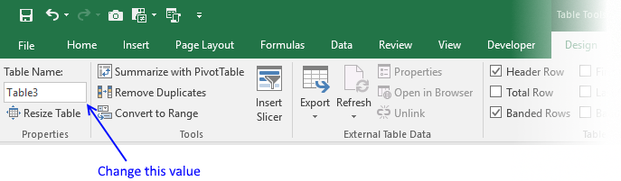
2. How to name an Excel Table
I recommend you give the table and table headers descriptive names, for example, it will be easier to identify cell references to Excel Tables in formulas. Cell references are called structured references and you can read about these in this article as well.
- Select a cell in your table
- Excel automatically navigates to tab "Design" on your ribbon
- Change table name
- Press Enter
3. How to manipulate Excel Table data
3.1 How to edit an Excel Table value
- Doublepress with left mouse button on any cell with left mouse button to start editing an Excel Table value.
- Use arrow keys to move the prompt between characters.
- Press Enter to apply changes or press CTRL + SHIFT + Enter to create an array formula.
3.2 How to delete an Excel Table value
- Press with left mouse button on with the left mouse button on any cell in the Excel Table to select it.
- Press Delete on the keyboard to remove the cell value.
3.3 How to add a row
- Press with left mouse button on with the left mouse button on any cell in the Excel Table to select it.
- Press the Tab key repeatedly until a new row is created.
A new row is created if you press the tab key with the lower right cell in the Excel Table selected. See the animated picture above.
Here is another way to create a new row.
- Select any cell right below the Excel Table the cell must be adjacent to the Excel Table for this to work.
- Type a value or a formula.
- Press Enter.
The Excel Table grows automatically when you add values adjacent to the Excel Table.
3.4 How to add a column
- Press with mouse on any cell adjacent to the Excel Table with the left mouse button to select it.
- Type a value or formula.
- Press Enter or CTRL + SHIFT + Enter.
The table expands automatically when you add values to adjacent cells, see the animated image above.
Add data to a cell adjacent to the table and the table expands automatically.
3.5 How to delete an Excel Table row
- Press with right mouse button on on one of the cells on the row you want to delete in the Excel Table.
- A popup menu appears, press with left mouse button on "Delete" on the popup menu.
- Another popup menu shows up, press with left mouse button on Table Rows.
This deletes the entire Excel Table row, it does not delete other values outside the Excel Table. At least not in Excel 365.
3.6 How to delete an Excel Table column
- Press with right mouse button on on any cell in an Excel Table. A popup menu appears.
- Press with mouse on "Delete" on the popup menu. Another popup menu shows up.
- Press with mouse on "Table Columns" .
3.7 How to delete an Excel Table and keep values

- Press with mouse on any cell in the Excel Table to select it. A tab named "Table Design" appears on the ribbon, this tab is not visible if not a cell in the Excel Table is sleected.
- Press with mouse on tab "Table Design" on the ribbon.
- Press with mouse on the "Convert to Range" button, see the image above.

The image above shows the Excel Table after converting to a normal range of cells. However, the cell formatting is still preserved.
Here is how to remove the cell formatting as well:
- Select the entire data set.
- Go to tab "Home" on the ribbon.
- Press with mouse on "Clear" button. A popup menu appears.
- Press with left mouse button on "Clear Formats".

4. How to sort an Excel Table
Sorting a table is easy, press with left mouse button on any black triangle located at each header, a menu appears allowing you to quickly sort data in a descending or ascending order.
An arrow next to the black triangle indicates sort order. Sort Z to A (descending) shows you an arrow pointing down.
You can also sort on multiple columns, follow these steps.
- Press with right mouse button on on a cell
- Press with left mouse button on Sort and then press with left mouse button on "Custom Sort..."
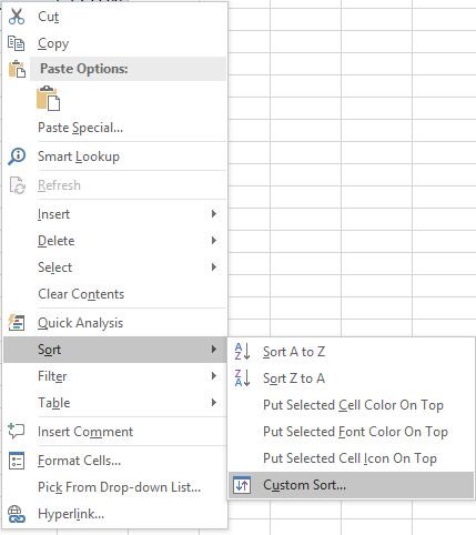
- Select column name to sort on and sort order then add more columns.
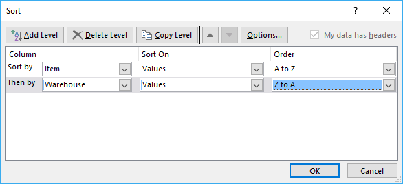
- Press with left mouse button on OK button to apply sort settings to table
The following article demonstartes how to sort a values in an excel defined table using a macro:
Recommended articles
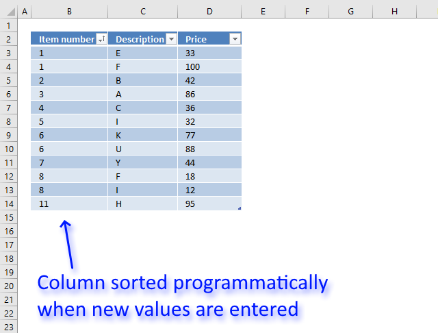
This article demonstrates how to sort a specific column in an Excel defined Table based on event code. The event […]
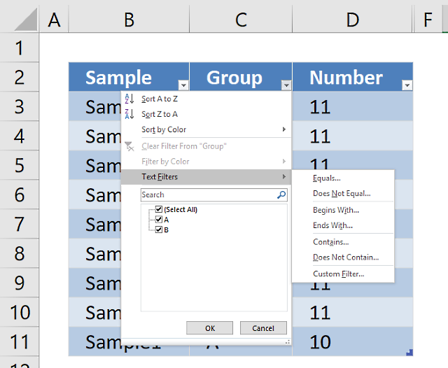
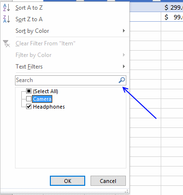
5. How to filter an Excel Table
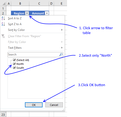
- Press with mouse on a black triangle next to any header
- Select values you want to filter
- Press with left mouse button on OK button
See animated picture below.
Excel allows you to apply filters to multiple columns easily, repeat above steps with another column.
Use the search field to quickly find the value you want to filter, see picture below.
6. How to insert a total to an Excel Table and sum using a condition
You can quickly sum values using table filtering.
Select a cell in the table, then go to tab "Design" on the ribbon.
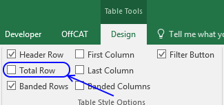
Press with left mouse button on "Checkbox" to enable "Total Row".
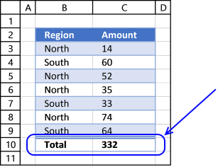
A row with totals appears on your table (332), see picture above.
Now filter the table, see instructions on picture below.
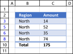
See how the total changes from 332 to 175.
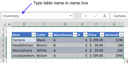
7. How do structured references work?
You are probably used to cell references like this one:
Creating a cell reference to a table column returns this instead, see picture below.
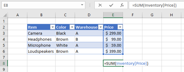
First the table name (Inventory) and then the column name enclosed with brackets [Price].
What is the purpose of structured references? The amazing thing with structured references is that if you add or remove values to a table the structured reference stays the same, no need to update cell references. In other words, they are dynamic.
7.1 Reference an entire Excel Table

The following structured reference returns the entire Excel Table including the column header names.
Formula in cell B9:
7.2 Reference Excel Table data

The following structured reference returns all Excel Table data, however, no the column header names.
Formula in cell B9:
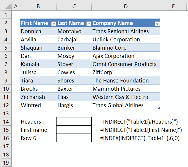
7.3 Reference all column headers

The following structured reference returns all Excel Table column header names.
Formula in cell B9:
7.4 Reference a column

The following structured reference returns all Excel Table data from a given column.
Formula in cell B9:

The following structured reference returns all Excel Table data from a given column including the column header name.
Formula in cell B9:
7.5 Reference a value on the same row

The following structured reference returns an Excel Table value from a given column but on the same row as the formula is entered on.
Formula in cell G4:
8. How to use a formula in an Excel Table
The following example demonstrates what happens if I type a formula in an excel table. I want to multiply cell E3 with F3 in cell G3, see animated picture below.
Excel creates these structured cell references in cell G3 if I type = (equal sig) and then press with left mouse button on cell E3, type * (asterisk) and then press with left mouse button on cell F3:
=[@['#]]*[@Price]
@ (at) means cell value on same row as formula.
Excel also calculates the remaining cells in column G automatically, see animated picture above.
Creating a reference to the entire excel table and headers returns this: =Inventory[#All]
A reference to data in table looks like this: =Inventory
A reference to a table column returns: =Inventory[Warehouse]
A reference to a column header only looks like this: =Inventory[[#Headers],[Warehouse]]
Back to top
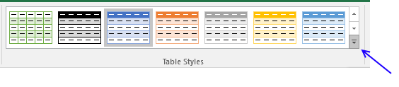
9. How to change Excel Table formatting
- Select a cell in excel table
- Go to tab "Design" on the ribbon
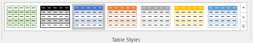
- Hover over a table style and see your table change
- If you like it press with left mouse button on it to select it
- Press with left mouse button on the black triangle to se even more table styles
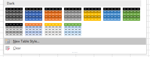
You can also build your own table style.
- Select a table cell
- Go to tab "Design"
- Press with left mouse button on black triangle
- Press with left mouse button on "New Table Style..."
- Enter a name for your table style
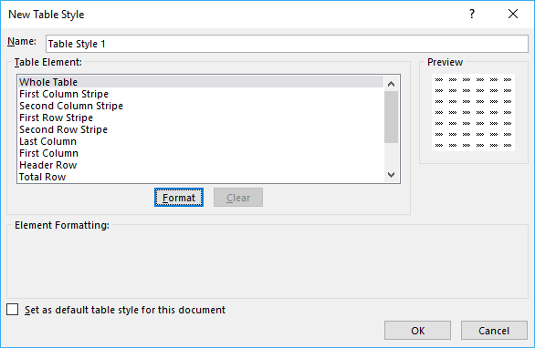
- Select a table element you want to change
- Press with left mouse button on "Format" button
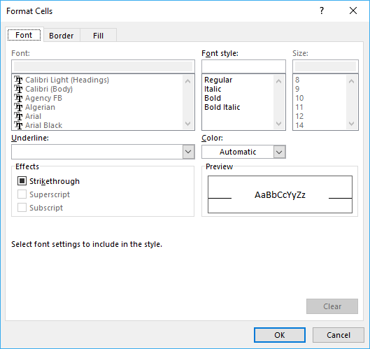
- Format as you like
- Press with left mouse button on OK button twice
10. How to show Excel Table totals
- Press with mouse on a cell in an excel table
- Go to tab "Design"
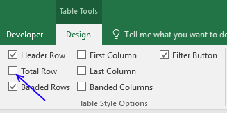
- Press with left mouse button on "Total Row" check box
- Press with left mouse button on cell G7 and then on black triangle
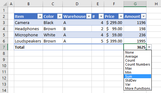
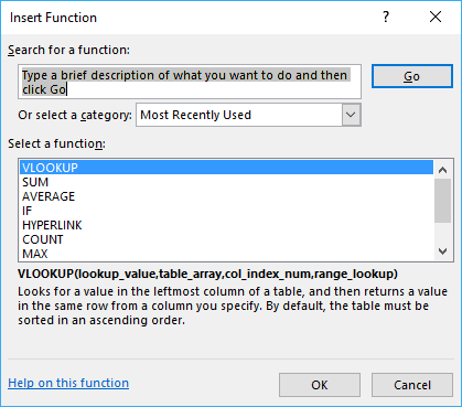
- You can change how value in cell G7 is calculated, the menu has these formulas: Average, Count, Count Numbers, Max, Min, Sum, StdDev, Var and More Functions.
- If you press with left mouse button on "More Functions" a dialog box opens with formulas to choose from.
11. List all tables in workbook - Named ranges
The Name Manager contains a list of all named ranges and Excel tables in your workbook.
- Press with left mouse button on the "Formula" tab on the ribbon.
- Press with left mouse button on "Name Manager" button.
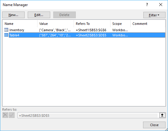
There are only Excel Tables in this workbook so the dialog box shows the Excel Table names, there are no named ranges in this workbook. See the image above.
12. How to link a chart to an Excel Table
Combine chart and table to make use of dynamic cell references while filtering data.
More details here: How to create a dynamic chart
Back to top
13. How to link a drop-down list to an Excel Table (Data validation)
The following animation shows you a data validation list linked to a table.
Read this post if you are interested in the details:
How to use a table name in data validation lists and conditional formatting formulas
Back to top
14. Working with a filtered Excel Table
If you try to use a filtered table as a data source in a formula you are in for trouble, see animated picture below.
As you can see above the SUM function sums all values in table regardless of filtered or not.
I have written a few articles about this:
- Highlight duplicates in a filtered excel defined table
- Count unique distinct values in a filtered table
- Highlight unique values in a filtered excel table
- Populate a list box with visible unique values from an excel table (vba)
- Highlight unique values in a filtered excel table
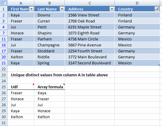
- Extract unique distinct values from a filtered table (udf and array formula)
- Vlookup visible data in a table and return multiple values
15. How to quickly find an Excel Table in a workbook
Excel lets you quickly focus on a table if you type the table name in the name box.
16. List Excel defined Tables in a workbook - VBA

The following macro inserts a new sheet to your workbook and lists all Excel defined Tables and corresponding Table headers in the active workbook.
16.1 Macro - VBA code
'Name macro
Sub ListTables()

'Declare variables and data types
Dim tbl As ListObject
Dim WS As Worksheet
Dim i As Single, j As Single

'Insert new worksheet and save to object WS
Set WS = Sheets.Add

'Save 1 to variable i
i = 1

'Go through each worksheet in the worksheets object collection
For Each WS In Worksheets

    'Go through all Excel defined Tables located in the current WS worksheet object
    For Each tbl In WS.ListObjects

        'Save Excel defined Table name to cell in column A
        Range("A1").Cells(i, 1).Value = tbl.Name

        'Iterate through columns in Excel defined Table
        For j = 1 To tbl.Range.Columns.Count

            'Save header name to cell next to table name
            Range("A1").Cells(i, j + 1).Value = tbl.Range.Cells(1, j)

        'Continue with next column
        Next j

        'Add 1 to variable i
        i = i + 1

    'Continue with next Excel defined Table
    Next tbl

'Continue with next worksheet
Next WS

'Exit macro
End Sub
16.2 List Excel Tables - example
Sheet1, 2 and 3 contain three tables.

16.3 Run macro
- Go to "Developer" tab
- Press with left mouse button on "Macros" button
- Press with left mouse button on "ListTables"
- Press with left mouse button on "Run"
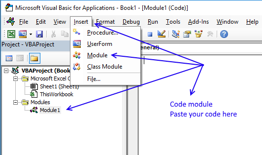
16.4 Where to copy macro

- Press Alt+F11 to open the VB Editor
- Press with left mouse button on "Insert" on the menu and then press with left mouse button on module.
- Copy above VBA code and paste to code module, see image above.
16.5 Get file
17. Extract rows where any cell is equal to a condition
How do I identify rows that have a specific cell value in an Excel defined table?

Array formula in B13:E15
How to create an array formula
- Select cell range B13:E15
- Copy/Paste above formula
- Press and hold Ctrl + Shift
- Press enter once
- Release all keys
Excel defined table
Table1 (B3:E6)
What is named ranges?
Array formula explanation
Step 1 - Find cells in named range matching criterion
=IFERROR(INDEX(Table1, SMALL(IF(Table1=$C$9, ROW(Table1)-MIN(ROW(Table1))+1, ""), ROW(Table1)-MIN(ROW(Table1))+1), COLUMN(Table1)-MIN(COLUMN(Table1))+1), "")
Table1=$C$9
becomes
B3:E6=$C$9
becomes
{East, AA, EE, HH; North, BB, AA, GG; South, CC, FF, DD; West, DD, CC, AA}= AA
becomes
{FALSE,TRUE,FALSE,FALSE,FALSE,FALSE,TRUE,FALSE,FALSE, FALSE,FALSE,FALSE,FALSE,FALSE,FALSE,TRUE}
Step 2 - Extract row numbers
=IFERROR(INDEX(Table1, SMALL(IF(Table1=$C$9, ROW(Table1)-MIN(ROW(Table1))+1, ""), ROW(Table1)-MIN(ROW(Table1))+1), COLUMN(Table1)-MIN(COLUMN(Table1))+1), "")
IF(Table1=$C$9, ROW(Table1)-MIN(ROW(Table1))+1, "")
becomes
IF({FALSE,TRUE,FALSE,FALSE,FALSE,FALSE,TRUE,FALSE,FALSE, FALSE,FALSE,FALSE,FALSE,FALSE,FALSE,TRUE}, {1,1,1,1;2,2,2,2;3,3,3,3;4,4,4,4}, "")
becomes
{"",1,"","";"","",2,"";"","","","";"","","",4}
Step 3 - Return the k-th smallest row number
SMALL(array,k) returns the k-th smallest number in this data set.
SMALL(IF(Table1=$C$9, ROW(Table1)-MIN(ROW(Table1))+1, ""), ROW(Table1)-MIN(ROW(Table1))+1)
becomes
SMALL({"",1,"","";"","",2,"";"","","","";"","","",4}, {1,1,1,1;2,2,2,2;3,3,3,3;4,4,4,4})
becmoes
{1,1,1,1;2,2,2,2;4,4,4,4}
Step 4 - Return matching records
INDEX(Table1, SMALL(IF(Table1=$C$9, ROW(Table1)-MIN(ROW(Table1))+1, ""), ROW(Table1)-MIN(ROW(Table1))+1), COLUMN(Table1)-MIN(COLUMN(Table1))+1)
becomes
INDEX(Table1, {1,1,1,1;2,2,2,2;4,4,4,4}, COLUMN(Table1)-MIN(COLUMN(Table1))+1)
becomes
INDEX(Table1, {1,1,1,1;2,2,2,2;4,4,4,4}, {1,2,3,4;1,2,3,4;1,2,3,4;1,2,3,4})
and returns:
{"East","AA","EE","HH";"North","BB","AA","GG";"West","DD","CC","AA"}
Get Excel *.xlsx file
search-for-a-string-in-excel-table.xlsx
18. Filter an Excel defined Table programmatically - VBA
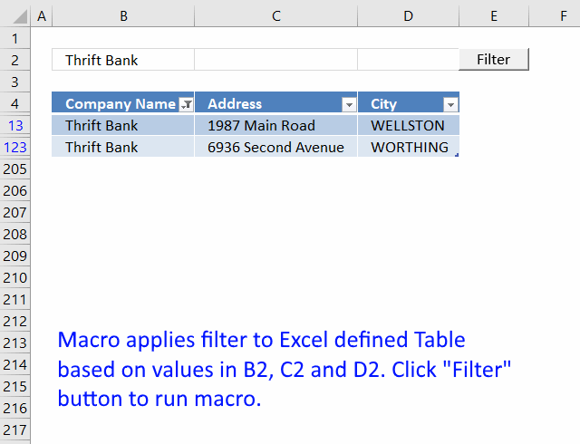
In this tutorial, I am going to demonstrate how to filter an Excel define Table through a VBA macro.
How it works
- Type a value in cell range B2, C2 or D2.
- Press Filter button
The table column below is instantly filtered. If the cell value is empty, no filter is applied.
VBA code
Sub TblFilter()

If Worksheets("Sheet1").Range("A2") <> "" Then
    Worksheets("Sheet1").ListObjects("Table1").Range.AutoFilter _
    Field:=1, Criteria1:="=" & Worksheets("Sheet1").Range("A2")
Else
    ActiveSheet.ListObjects("Table1").Range.AutoFilter Field:=1
End If

If Worksheets("Sheet1").Range("B2") <> "" Then
    Worksheets("Sheet1").ListObjects("Table1").Range.AutoFilter _
    Field:=2, Criteria1:="=" & Worksheets("Sheet1").Range("B2")
Else
    ActiveSheet.ListObjects("Table1").Range.AutoFilter Field:=2
End If

If Worksheets("Sheet1").Range("C2") <> "" Then
    Worksheets("Sheet1").ListObjects("Table1").Range.AutoFilter _
    Field:=3, Criteria1:="=" & Worksheets("Sheet1").Range("C2")
Else
    ActiveSheet.ListObjects("Table1").Range.AutoFilter Field:=3
End If

End Sub
Where to copy vba code?
- Copy above VBA macro (CTRL + c)
- Press Alt+F11 to open the Visual Basic Editor.
- Press with left mouse button on "Insert" on the menu.
- Press with left mouse button on "Module" to create a module.
- Paste code to module (CTRL + v)
- Exit VBE and return to Excel.
How to create a button
- Press with left mouse button on "Developer" tab.
- Press with left mouse button on "Insert" button.
- Create a button (Form Control).
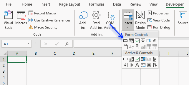
- Press with left mouse button on and drag on your worksheet to create the button.
- Press with right mouse button on on your new button.
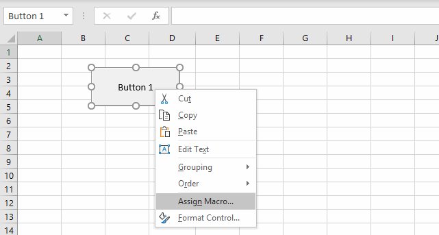
- Select a macro to assign.
- Press with left mouse button on OK button.
The assigned macro is rund when the user press with left mouse button ons on the button.
19. Basic Invoice Template
In my workbook I have three worksheets; "Customer", "Vendor" and "Payment".
In the Customer sheet I have a table, tblCustomer, where I add new customers. Similarly, in the Vendor sheet I have a table, tblVendor, where I add new vendors.
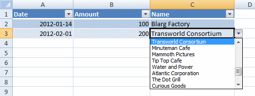
In the Payment sheet I have a table, tblPayment, where i have three columns; Date, Amount and Name.
Now, here is what I want to do; In the Name column of the tblPayment, I want to create a drop down list in each cell, which would contain all the names from tblCustomer[Name] and tblVendor[Name].
This way I can fill in the Date, Amount and then select one of all the names available in the drop down list of my Name cell. Is this possible without using VB code or any macro? If so, please help me out with this.
Answer:
Yes, it is possible to merge values from both Excel defined Tables without using VBA, however, you need a "Calculation" sheet containing a formula that extracts the values from both sources to one distinct column.
A dynamic named range will then be used in order to get all values from the calculation sheet and inserted to a drop-down list.
Sheet: Customer

Sheet: Vendor

Sheet:Calc

Array formula in cell A2:
How to create an array formula
- Copy (Ctrl + c) above array formula
- Select cell A2
- Paste (Ctrl + v)
- Press and hold Ctrl + Shift
- Press Enter once
- Release all keys
How to copy array formula
- Select cell A2
- Copy (Ctrl + c)
- Select cell range A3:A100
- Paste (Ctrl + v)
Create named range

Named range formula:
Sheet: Payment
Create drop down list
- Select cell C2
- Go to "Data" tab
- Press with left mouse button on "Data validation"

- Select List
- Type =Names in Source field
- Press with left mouse button on OK
Get excel file *.xlsx
20. Filter an Excel defined Table based on selected cell - VBA

In this post I am going to demonstrate how to quickly apply a filter to a table. I am using the selection change event to apply the filter. Press with mouse on a cell in a table and the cell value is instantly used as a filter in the current table column.
Select a cell outside the table and all table filters are removed. Unfortunately, you can't select multiple cells in a table column in this macro.
Nothing in the table is selected, see picture above.

Cell B4 is selected in the picture above and the Excel defined Table is instantly filtered based on cell B4.

This example shows cell C4 selected. Now are both values in cell B4 and C4 are now used as filtering parameters, simply press with left mouse button on a cell outside the Excel defined Table to clear filter conditions.
VBA Event code
The following Event code is rund every time a cell is selected.
'To use this Event the name must be Worksheet_SelectionChange(ByVal Target As Range)
Private Sub Worksheet_SelectionChange(ByVal Target As Range)

'Declare variables and data types
Dim ACell As Range
Dim ActiveCellInTable As Boolean
Dim Scol As Single

'Enable error handling
On Error Resume Next

'Save cell to object ACell
Set ACell = Selection

Save Boolean value TRUE or FALSE to ActiveCellInTable  based on if Table name is empty or not.
ActiveCellInTable = (ACell.ListObject.Name <> "")

'Disable error handling
On Error GoTo 0

'Check if ActiveCellInTable equals to False meaning if selected cell is outside the Excel defined Table
If ActiveCellInTable = False Then

   'Go through ListObjects (Excel defined Tables)
   For i = 1 To ActiveSheet.ListObjects.Count

      'Iterate through columns
      For j = 1 To ActiveSheet.ListObjects(i).Range.Columns.Count

          'Clear filter conditions for each column
          ActiveSheet.ListObjects(i).Range.AutoFilter Field:=j
      Next j
   Next i

   'Stop Event code
   Exit Sub
End If

'Make sure that only one cell is selected or stop event code
If Selection.Cells.Count > 1 Then Exit Sub

'Calculate relative column number in the Excel defined Table
Scol = Selection.Column - ACell.ListObject.Range.Column + 1

'Apply filter condition to given column
ActiveSheet.ListObjects(ACell.ListObject.Name).Range.AutoFilter _
Field:=Scol, Criteria1:="=" & Selection

End Sub
Where to copy the code?
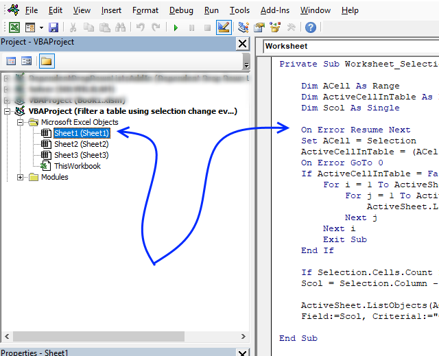
- Press Alt+F11 to open the VB Editor
- Double press with left mouse button on the sheet where the Excel defined Table is located in the project explorer window
- Copy / Paste vba code to sheet module
- Return to excel
21. Use a calendar to filter an Excel defined Table
This article demonstrates how to filter an Excel defined Table based on the selected cell in a calendar. The calendar highlights dates containing appointments or events, the clear button below the calendar deletes all filter conditions.
My previous post Excel calendar (vba) used a formula to extract events based on selected cell, this article shows you event code and a macro to filter the Excel defined Table itself.
How to use this workbook
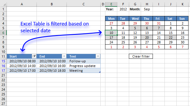
The animated image below shows what happens with the Excel Table when you select different cells in the calendar, it also shows what happens when you press with left mouse button on the "clear filter" cell.

The Excel defined table and calendar, unfortunately, have to be located like the image shows above. The Excel Table will filter out calendar rows if they are next to each other.
I would certainly have liked the calendar above the table but that makes it impossible to adjust the calendar's cell widths to the same size.
How I created this workbook
The calendar is dynamic meaning it changes automatically based on the selected year and month.
Create calendar
See steps in my previous post.
Conditional formatting
For some reason I don't understand, a table name is not allowed in a conditional formatting formula . I ended up creating a named range:

Update: You can use the INDIRECT function in order to use Excel defined Tables in Conditional Formatting formulas, you can read more about it here: How to use a Table name in Data Validation Lists and Conditional Formatting formulas
Conditional formatting formula:

Conditional Formatting formula for highlighting days containing events:
See remaining steps in my previous post.
Vba code
'Event code that is triggered when the user selects any cell in cell range E4:K9
Private Sub Worksheet_SelectionChange(ByVal Target As Range)

'Check if selected cell is in cell range E4:K9 and the number of selected cells are 1
If Not Intersect(Target, Range("E4:K9")) Is Nothing And Target.Cells.Count = 1 Then

'Apply a filter to first column in Excel table named Table1 based on selected cell's date
ActiveSheet.ListObjects("Table1").Range.AutoFilter _
Field:=1, Criteria1:=">=" & Target.Value, Operator:=xlAnd, Criteria2:="<" & Target.Value + 1
SortTable

'Clear filter if cell G11 is selected
ElseIf Not Intersect(Target, Range("G11")) Is Nothing Then
ActiveSheet.ListObjects("Table1").Range.AutoFilter Field:=1

'Run macro SortTable
SortTable
End If
End Sub
Sub SortTable()
'Sort table in an ascending order based on first column
With ActiveWorkbook.Worksheets("Calendar").ListObjects("Table1").Sort
.SortFields.Clear
.SortFields.Add Key:=Range("Table1[[#All],[Start]]"), SortOn:=xlSortOnValues, Order:= _
xlAscending, DataOption:=xlSortNormal
.Header = xlYes
.MatchCase = False
.Orientation = xlTopToBottom
.SortMethod = xlPinYin
.Apply
End With
End Sub
Where to put the VBA code?
- Press with right mouse button on on the sheet name, it is located at the very bottom of the Excel screen.

- Press with left mouse button on "View code".

- Paste event code to sheet module.
- Return to excel.
How to add new records to the table
- Select the last cell in the table

- Press Tab key

- Enter new values
New records are also highlighted in the calendar. Make sure you have selected the correct month to be able to see them.
Recommended blog posts
Filter a table using the selection change event
Extract unique distinct values from a filtered table (udf and array formula)
Quickly filter a column in an excel table
Table category
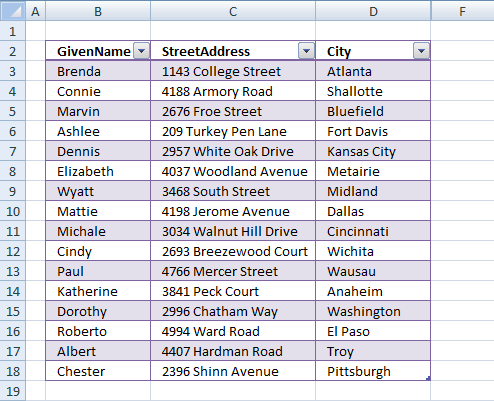
Table of Contents How to compare two data sets - Excel Table and autofilter Filter shared records from two tables […]
This article demonstrates different ways to reference an Excel defined Table in a drop-down list and Conditional Formatting formulas. The […]
This article demonstrates two formulas that extract distinct values from a filtered Excel Table, one formula for Excel 365 subscribers […]
How to use Excel Tables
12 Responses to “How to use Excel Tables”
Leave a Reply
How to comment
How to add a formula to your comment
<code>Insert your formula here.</code>
Convert less than and larger than signs
Use html character entities instead of less than and larger than signs.
< becomes < and > becomes >
How to add VBA code to your comment
[vb 1="vbnet" language=","]
Put your VBA code here.
[/vb]
How to add a picture to your comment:
Upload picture to postimage.org or imgur
Paste image link to your comment.
Thank you very much. This solution has worked nicely.
Now, say if I have 1000 names alltogether. I guess I'll have to copy the array formula upto cell A1001. Also, I will have to increase the $A$500 upto $A$1001 in the Named Range Formula. Is that right?
Thanks again.
Hey Oscar,
I have done a slight change in my workbook. In Sheet:Calc, I have made a table in Column A and named it tblAllNames. Then I copied the array formula in its first row and adjusted the table rows as far as I needed (by pulling down the bottom right corner of the table). This way the formula copies itself in all the rows. Also, I can add names, which don’t exist in either of the Customer or Vendor tables, such as Bank Name or Employee Name, etc. I do have to remember not to sort this table because I tried that and it messed up things.
Then after this I created a Named range called AllNames and simply replaced the range by table name.
In its formula box I typed: =OFFSET(tblAllNames, 0, 0, MAX(IF(tblAllNames"", ROW(tblAllNames), "A"))-1).
This worked fine.
Can you please explain how this formula works? Why do you have “A” in it?
By the way, what if I make another table called tblEmployee and want to add all employee names to my drop down list as well . I’m sure a lot of things are going to change in the array formula.
Rattan,
In its formula box I typed: =OFFSET(tblAllNames, 0, 0, MAX(IF(tblAllNames"", ROW(tblAllNames), "A"))-1).
This worked fine.
Can you please explain how this formula works? Why do you have “A” in it?
You can also use "". The "A" is just a random letter. Max function handles only numerical values, remaining values are ignored.
Explaining the named range formula
The formula gets all values in tblAllNames. I can´t use counta function in this case.
Step 1 - Convert nonempty values to row numbers
IF(tblAllNames<>"", ROW(tblAllNames), "A")
Step 2 - Get the largest row number
MAX(IF(tblAllNames<>"", ROW(tblAllNames), "A"))
Step 3 - Get values from cell range
=OFFSET(tblAllNames, 0, 0, MAX(IF(tblAllNames<>"", ROW(tblAllNames), "A"))-1)
By the way, what if I make another table called tblEmployee and want to add all employee names to my drop down list as well . I’m sure a lot of things are going to change in the array formula.
Change formula in sheet Calc to the formula found in this blog post:
Merge three columns into one list in excel
" a table name is not allowed in a conditional formatting formula."
It is, but it has to be used like this:
=INDIRECT("Table1[Start]")
David Hager,
Thanks!!
[...] Make sure you have selected the correct month to be able to see them.Recommended blog postsFilter a table using the selection change eventExtract unique distinct values from a filtered table (udf and array formula)Quickly filter a column [...]
This file Table and calendar.xlsm, is not workink for me.
Yoram,
What happens?
Dear sir,
I have saved invoice with Party No in A column and Inv No in B column and untill N column the rest of the invoice data.
my qstn is when i enter Party no in textbox the all the invoices relating to that party should appear in listbox. how can i do that?
Hi,
I deal with this issue constantly, and I cant seem to find any solution for this. I hope you can help me out. I have a set of daily events for 80 days straight. I have written down events from day 1-80. I am looking for a file where I set the starting date, month and year, and the file creates a calendar (or a list) from day 1 for the following 80 days. Then export the calendar to iCal or googleCal.
I need help in coding having below conditions while filter items there are about 1 lakh+ records in a table without any additional column in table.
1. Select all between 1000 and 1500
2. Select 1800,1820,1825
3. Select all between 2000 and 2200
4. Select all above 2800
Is there a way this can be done with out a VBA, my work has restricted access to VBA content.
For example can you take a month, January, and then show all the scheduled appointments for January just like the example above? No need to click on the date in the calendar to see appointments, just a month at a glance? With the highlighted calendar above it?