Extract a unique distinct list sorted from A to Z
This article demonstrates Excel formulas that allows you to list unique distinct values from a single column and sort them alphabetically in both Excel 365 and older Excel versions.
What are unique distinct values?
Unique distinct values refer to a set of values that are present in a dataset or a list, without any duplicates. In other words, it's a collection of values where each value appears only once.
For example, let's say you have a list of colors: Red, Blue, Green, Red, Yellow, Blue, Green, Purple
The unique distinct values in this list would be: Red, Blue, Green, Yellow, Purple
Notice that the duplicates (Red, Blue, and Green) are removed, and only one instance of each value is kept. This is useful in data analysis and processing, as it helps to eliminate redundant information and provide a more concise view of the data.
Will these formulas work with source cell ranges larger than 1 column?
No, they won't. See this article: Extract unique distinct values from a multi-column cell range
Table of Contents
- Extract a unique distinct list sorted from A to Z
- Unique distinct list sorted alphabetically based on a condition - Earlier Excel versions
- Unique distinct list sorted alphabetically based on a condition - Excel 365
- Unique distinct list sorted alphabetically based on a numerical range - Earlier Excel versions
- Unique distinct list sorted alphabetically based on a numerical range - Excel 365
- Get *.xlsx file
- Extract a unique distinct list and ignore blanks
- Extract a unique distinct list and ignore blanks (Excel 365)
- Extract a unique distinct list and ignore blanks (UDF)
- Get Excel file
- Extract a unique distinct list sorted from A to Z and ignore blanks - earlier Excel versions
- Create a unique distinct sorted list containing both numbers and text removing blanks with a condition - earlier Excel versions
- List unique distinct sorted values removing blanks based on a condition - Excel 365
- Create a unique distinct sorted list containing both numbers and text removing blanks with a condition - Excel 365
- Create unique distinct list sorted based on text length
1. Extract a unique distinct list sorted from A to Z
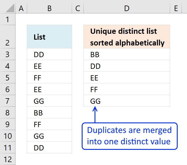
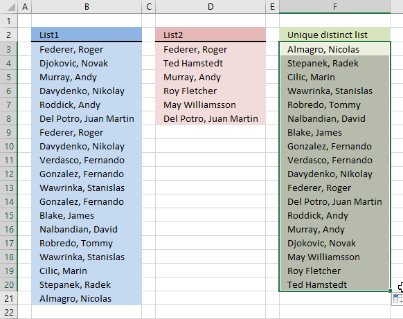
The array formula in cell D3 extracts unique distinct values sorted A to Z, from column B to column D. Unique distinct values are all values except duplicates.
Example, in column B value "DD" exists twice in cell B3 and B11. In column D value "DD" exists only once since it is a unique distinct list.
Update 2020-12-09, the formula below is for Excel 365 subscribers:
You can find an explanation here: Extract unique distinct values sorted from A to Z and other examples here: How to use the UNIQUE function
Use the array formula below if you own an earlier Excel version.
Array formula in cell D3:
Watch a video that explains how to use it and how it works:
Learn how to filter values with a condition and return unique distinct values sorted from A to Z:
Recommended articles
This article demonstrates how to extract unique distinct values based on a condition and also sorted from A to z. […]
How to create an array formula
- Double press with left mouse button on cell D3
- Copy (Ctrl +c) amd paste (Ctrl+v) above formula to cell D3
- Press and hold Ctrl + Shift simultaneously
- Press Enter once
- Release all keys
The formula in the formula bar should now look like this: {=formula}
Don't enter the curly brackets yourself, they appear automatically.

Recommended articles

Array formulas allows you to do advanced calculations not possible with regular formulas.
How to copy array formula
- Select cell D3
- Copy cell (Keyboard shortcut: Ctrl + c)
- Select cell range D4:D7
- Paste (Keyboard shortcut: Ctrl + v)
Explaining array formula in cell
Step 1 - Identify values not yet shown above current cell
The COUNTIF function counts the number of times a value exists in a cell range.
Cell range $D$2:D2 changes as the formula is copied down to cells below. This makes it possible to avoid duplicate values in the list.
COUNTIF($D$2:D2,$B$3:$B$11)=0 returns {TRUE; TRUE; TRUE; ... ; TRUE}
Step 2 - Create an array with a ranking sort number
COUNTIF($B$3:$B$11,"<"&$B$3:$B$11) returns {1;3;5;3;7;0;5;7;1}
Step 3 - Convert array with not displayed values to an array containing rank numbers
The IF function converts not yet displayed values into alphabeically ranked numbers.
IF(COUNTIF($D$2:D2,$B$3:$B$11)=0,COUNTIF($B$3:$B$11,"<"&$B$3:$B$11),"") returns {1;3;5;3;7;0;5;7;1}
Step 4 - Find the smallest value in array
The SMALL function extracts the smallest number in the array.
SMALL(IF(COUNTIF($D$2:D2, $B$3:$B$11)=0, COUNTIF($B$3:$B$11,"<"&$B$3:$B$11), ""),1) returns 0.
Recommended articles
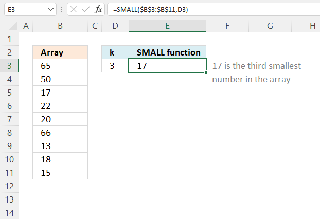
The SMALL function lets you extract a number in a cell range based on how small it is compared to the other numbers in the group.
Step 5 - Find relative position in the array
The MATCH function finds the position of the next alphabetically sorted value.
MATCH(SMALL(IF(COUNTIF($D$2:D2, $B$3:$B$11)=0, COUNTIF($B$3:$B$11,"<"&$B$3:$B$11),""), 1),COUNTIF($B$3:$B$11, "<"&$B$3:$B$11), 0) returns 6.
Step 6 - Return value in data based on row coordinate
The INDEX function returns a value based on row and column number.
INDEX($B$3:$B$11, MATCH(SMALL(IF(COUNTIF($D$2:D2, $B$3:$B$11)=0, COUNTIF($B$3:$B$11, "<"&$B$3:$B$11), ""), 1), COUNTIF($B$3:$B$11, "<"&$B$3:$B$11), 0))
returns BB in cell D3.
Get excel *.xlsx file
Unique distinct list sorted alphabetically.xlsx
2. Unique distinct list sorted alphabetically based on a condition - earlier Excel versions

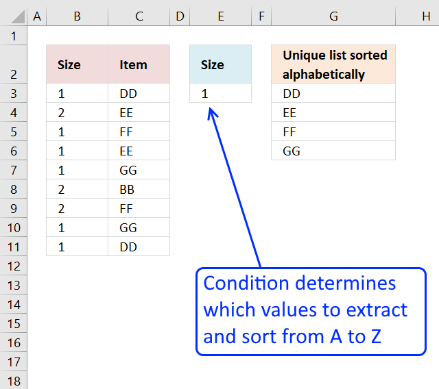
The image above demonstrates a formula in cell G6 that extracts unique distinct values only if the corresponding value on the same row meets a given condition.
The array formula below is for earlier Excel versions, it filters values in column C based on the value in cell E3, the output is a sorted unique distinct list in cell G3 and cells below.
Array formula in cell G3:
Recommended post
Recommended articles
2.1 How to create an array formula
- Double press with left mouse button on cell G3.
- Copy (Ctrl + c) and paste (Ctrl + v) array formula to cell.
- Press and hold CTRL + SHIFT simultaneously.
- Press Enter once.
- Release all keys.
There is now a beginning and ending curly bracket in the formula bar, like this: {=formula}
Don't enter these characters yourself, they appear automatically if you completed the above steps.
2.2 Explaining array formula in cell G3
Step 1 - Count values
The COUNTIF function counts values based on a condition or criteria.
COUNTIF(range, criteria)
The range argument contains a cell reference that is both relative and absolute meaning it grows when the formula is copied to cells below. This makes the formula aware of the previous values above.
COUNTIF($G$2:G2, $C$3:$C$11) returns {0;0;0;0;0;0;0;0;0}. 0 (zero) means that no cells meet the given condition.
Step 2 - Check if values in array equals 0 (zero)
The equal sign compares the values in the array to 0 (zero). The output is a boolean value TRUE or FALSE.
COUNTIF($G$2:G2, $C$3:$C$11)=0 returns {TRUE; TRUE; TRUE; ... ; TRUE}.
Step 3 -
$B$3:$B$11=$E$3
Step 4 -
COUNTIF($G$2:G2, $C$3:$C$11)=0)*($B$3:$B$11=$E$3)
Step 5 -
IF((COUNTIF($G$2:G2, $C$3:$C$11)=0)*($B$3:$B$11=$E$3), COUNTIF($C$3:$C$11, "<"&$C$3:$C$11), "")
Step 6 -
SMALL(IF((COUNTIF($G$2:G2, $C$3:$C$11)=0)*($B$3:$B$11=$E$3), COUNTIF($C$3:$C$11, "<"&$C$3:$C$11), ""), 1)
Step 7 -
MATCH(SMALL(IF((COUNTIF($G$2:G2, $C$3:$C$11)=0)*($B$3:$B$11=$E$3), COUNTIF($C$3:$C$11, "<"&$C$3:$C$11), ""), 1), COUNTIF($C$3:$C$11, "<"&$C$3:$C$11), 0)
Step 8 -
INDEX($C$3:$C$11, MATCH(SMALL(IF((COUNTIF($G$2:G2, $C$3:$C$11)=0)*($B$3:$B$11=$E$3), COUNTIF($C$3:$C$11, "<"&$C$3:$C$11), ""), 1), COUNTIF($C$3:$C$11, "<"&$C$3:$C$11), 0))
Read my explanation here: Create a unique distinct alphabetically sorted list, extracted from a column
Recommended reading:
Recommended articles
3. Unique distinct list sorted alphabetically based on a condition - Excel 365

Update 17 December 2020, the new FILTER, UNIQUE, and SORT functions are now available for Excel 365 users.
The image above demonstrates a dynamic array formula that works only in Excel 365. Despite its name you simply enter it as a regular formula.
It filters values from column C based on the corresponding values in column B given the condition in cell E3. The output in cell G3 is a sorted unique distinct list from A to Z.
This is entered as a regular formula, however, it returns an array of values and extends automatically to cells below and to the right. Microsoft calls this a dynamic array and spilled array.
3.1 Explaining Excel 365 formula
Step 1 - Extract values based on a condition
The FILTER function extracts values based on a condition.
FILTER(C3:C11, E3=B3:B11)
Step 2 - Extract unique distinct values
The UNIQUE function returns an array of unique distinct values meaning duplicates are merged into one distinct value.
UNIQUE(FILTER(C3:C11, E3=B3:B11))
Step 3 - Sort values from A to Z
The SORT function returns an array of values sorted from A to Z in its default state.
SORT(UNIQUE(FILTER(C3:C11, E3=B3:B11)))
4. Unique distinct list sorted alphabetically based on a numerical range - Earlier Excel versions

The image above shows a formula in cell H3 that extracts values from column C it the corresponding numbers in column B meet a condition based on a numerical range specified in cells F3:F4.
The output in cell H3 and cells below as far as needed is a sorted unique distinct list from A to Z. Unique distinct values are all values, however, duplicate values are merged into one distinct value.
Formula in cell H3:
=INDEX($C$3:$C$11, MATCH(SMALL(IF((COUNTIF($H$2:H2, $C$3:$C$11)=0)*($B$3:$B$11>=$F$3)*($B$3:$B$11<=$F$4), COUNTIF($C$3:$C$11, "<"&$C$3:$C$11), ""), 1), COUNTIF($C$3:$C$11, "<"&$C$3:$C$11), 0))
4.1 Explaining formula
5. Unique distinct list sorted alphabetically based on a numerical range - Excel 365

Formula in cell H3:
=SORT(UNIQUE(FILTER(C3:C11,(F3<=B3:B11)*(F4>=B3:B11))))
5.1 Explaining Excel 365 formula
Step 1 -
F3<=B3:B11
Step 2 -
F4>=B3:B11
Step 3 -
(F3<=B3:B11)*(F4>=B3:B11)
Step 4 -
FILTER(C3:C11,(F3<=B3:B11)*(F4>=B3:B11))
Step 5 -
UNIQUE(FILTER(C3:C11,(F3<=B3:B11)*(F4>=B3:B11)))
Step 6 -
SORT(UNIQUE(FILTER(C3:C11,(F3<=B3:B11)*(F4>=B3:B11))))
6. Get Excel file
7. Extract a unique distinct list and ignore blanks
![]()
Question: How do I extract a unique distinct list from a column containing blanks?
Answer: Cell range B3:B12 contains several blank cells. The following formula in cell D3 extracts unique distinct values from cell range B3:B12. Unique distinct values are all values except duplicates are merged into one distinct value.
Formula in D3:
Copy cell B2 and paste to cells below.
7.1 Explaining the LOOKUP formula in cell D3
Step 1 - Check cell range B3:B12 for non-empty cells
If a cell contains a value TRUE is returned. The following line is a logical expression, cells not equal to nothing return TRUE. The less and larger than characters are logical operators that evaluates to boolean values, True or False.
$B$3:$B$12<>""
returns {TRUE;TRUE; ... ;TRUE}
Step 2 - Ignore duplicate cells
The COUNTIF function counts cells that equal a condition or any of the supplied criteria. The first argument has both an absolute and relative cell reference. This allows the cell range to grow when cell B3 is copied to cells below as far as needed.
COUNTIF($D$2:D2, $B$3:$B$12)=0
The equal sign is also a logical operator like the less and greater signs, it evaluates tor True or False.
{0;0;0;0;0;0;0;0;0;0}=0
returns {TRUE; TRUE; ...; TRUE}
Recommended articles

Counts the number of cells that meet a specific condition.
Step 3 - Multiply arrays
Multiplying boolean values is the same as applying OR logic to each value based on their position.
The first value in the first array is True and in the second array is also True. True * True equals 1.
The other possibilties are:
- True * False = 0 (zero)
- False * True = 0 (zero)
- False * False = 0 (zero)
The boolean equivalent to True is 1 and False is 0 (zero).
(COUNTIF($D$2:D2, $B$3:$B$12)=0)*($B$3:$B$12<>"")
returns {1; 1; 0; 1; 1; 1; 0; 1; 1; 1}
Step 4 - Divide 1 by the array
The reason I am dividing 1 with the array is to replace 0 (zero) with the #DIV/0. The LOOKUP function will ignore the #DIV/0 errors, shown in the next step.
1/((COUNTIF($D$2:D2, $B$3:$B$12)=0)*($B$3:$B$12<>""))
returns {1; 1; #DIV/0!;... ; 1}
Step 5 - Find last match in array and return corresponding value
LOOKUP(2, 1/((COUNTIF($D$2:D2, $B$3:$B$12)=0)*($B$3:$B$12<>"")), $B$3:$B$12)
returns "EE" in cell D3.
Recommended articles
Extract a unique distinct list from two columns
Vlookup – Return multiple unique distinct values
Extract a unique distinct list sorted from A to Z
Extract a unique distinct list from three columns
Extract unique distinct values from a multi-column cell range
Extract unique distinct values A to Z from a range and ignore blanks
Category 'Unique distinct values'
8. Extract a unique distinct list and ignore blanks - Excel 365
![]()
Update 10th December 2020: Excel 365 subscribers can now use this regular formula in cell D3.
There is no need to use absolute cell references with formulas that return a dynamic array, however, it is crucial that you use them with the first formula above, as shown.
Note that the formula above deploys an array of values to the appropriate cell range. If any of the cells below are populated cell D3 returns a #SPILL! error.
Check out how the Excel 365 formula works here:
Extract unique distinct values ignoring blanks
Recommended articles
FILTER function | UNIQUE function | LET function | XMATCH function | XLOOKUP function | Excel Function Library
9. Extract a unique distinct list and ignore blanks (UDF)

The image above shows a User Defined Function that extracts unique distinct values from a specific cell range.
What is a unique distinct value?
Unique distinct values are all values, however, duplicate values are merged into one distinct value. In other words, there are no duplicate values in the extracted list.
What is a User Defined Function (UDF)?
A UDF is a custom function that you can create yourself using Visual Basic for Applications (VBA) code. The code must be inserted into a code module in your workbook before you can use the custom function.
Formula in cell D3:
9.1 User Defined Function Syntax
FilterUniqueSort(rng)
9.2 User Defined Function arguments

rng - A reference to a cell range you want to extract values from. The example above uses cell reference B3:B12.
9.3 VBA code
'Name User Defined Function and define paremeter
Function FilterUniqueSort(rng As Range)

'Dimension variables and declare data types
Dim ucoll As New Collection, Value As Variant, temp() As Variant
Dim iRows As Single, i As Single

'Redimension array variable
ReDim temp(0)

'Enable error handling
On Error Resume Next

'Iterate through each value in range
For Each Value In rng

'Check if number of characters in value is greater than 0 (zero), if true add value to collection ucoll
If Len(Value) > 0 Then ucoll.Add Value, CStr(Value)

'Continue with next value
Next Value

'Disable error handling
On Error GoTo 0

'Iterate through each value in collection ucoll
For Each Value In ucoll

'Save value to last container in array variable temp
temp(UBound(temp)) = Value

'Add new container to array variable temp
ReDim Preserve temp(UBound(temp) + 1)

'Next value
Next Value

'Remove last container in array variable temp
ReDim Preserve temp(UBound(temp) - 1)

'Transpose values in array variable temp and return those values to worksheet
FilterUniqueSort = Application.Transpose(temp)

End Function
9.4 Where to put the code?

- Press shortcut keys Alt + F11 to open the Visual Basic Editor (VBE).
- Press the left mouse button on "Insert" on the menu, see the image above. A pop-up menu appears.
- Press the left mouse button on "Module" to create a module to your workbook.
- Copy (Ctrl + c) above VBA code
- Paste (Ctrl +v) to the code module, see the image above.
- Return to Excel.
Recommended reading
Extract unique distinct values from a filtered Excel defined Table [UDF and Formula]
Substitute multiple text strings [UDF]
SUMIF across multiple sheets [UDF]
List files in a folder and subfolders [UDF]
Category 'User Defined Functions'
10. Excel file
11. Extract a unique distinct list sorted from A to Z ignore blanks
![]()
The image above demonstrates a formula in cell D3 that extracts unique distinct numbers and text values sorted from A to Z and also ignores blank cells.
Array formula in cell D3:
How to create an array formula
- Copy above array formula
- Select cell D3
- Press with left mouse button on in formula bar

- Paste formula (Ctrl + v)
- Press and hold Ctrl + Shift
- Press Enter
How to copy array formula
Copy cell B2 and paste it down as far as needed.
Explaining formula in cell D3
There are two formulas in the IFERROR function, when the first formula is running out of numbers to return the second formula starts extracting text values.
IFERROR( formula1, formula2)
Step 1 - Prevent extracting duplicate numbers
The COUNTIF function counts cells in cell range based on a condition or criteria. If the value is equal to 0 then it has not been displayed yet. The first cell reference grows when the cell is copied to cells below, this makes the formula aware of previously displayed value above the current cell.
COUNTIF($D$2:D2,$B$3:$B$16)=0)
and returns {TRUE; TRUE; ... ; TRUE}
Step 2 - Identify numbers in column
The ISNUMBER function returns TRUE if value is a number.
ISNUMBER($B$3:$B$16)
and returns {FALSE; TRUE; ... ; FALSE}
Step 3 - Multiply arrays
Both arrays must return TRUE for the logical expression to return TRUE. In ordeer to achieve AND logic I multiply the arrays. TRUE * TRUE = TRUE, TRUE * FALSE = FALSE and FALSE * FALSE = FALSE.
(COUNTIF($D$2:D2, $B$3:$B$16)=0)*ISNUMBER($B$3:$B$16)
and returns {0;1;1;0;0;0;0;0;1;0;0;1;0;0}. 0 (zeros is the equivalent to FALSE and any other number is equal to boolean TRUE.
Step 4 - Replace TRUE with numbers in column
The IF function returns one value (argument2) if TRUE and another (argument3) if FALSE. The IF function returns "A" if logical expression is FALSE, this makes the SMALL function ignore the text value in the next step.
IF((COUNTIF($D$2:D2, $B$3:$B$16)=0)*ISNUMBER($B$3:$B$16), $B$3:$B$16, "A")
and returns {"A";8;12;"A";"A";"A";"A";"A";9;"A";"A";9;"A";"A"}.
Step 5 - Extract smallest number
To be able to return a new value in a cell each I use the SMALL function to filter numbers from smallest to largest.
SMALL(IF((COUNTIF($D$2:D2, $B$3:$B$16)=0)*ISNUMBER($B$3:$B$16), $B$3:$B$16, "A"), 1)
becomes
SMALL({"A";8;12;"A";"A";"A";"A";"A";9;"A";"A";9;"A";"A"}, 1)
and returns 8 in cell D3.
Explaining formula in cell D6
Step 1 - Prevent duplicates and only extract text values
This step and forward explains how to extract text values. We begin with cell D6 which is the first cell that extracts text values in our example. The ISTEXT function returns TRUE if value is a text value. The IF function returns a number representing the rank order if the list were sorted from A to Z.
IF(ISTEXT($B$3:$B$16)*(COUNTIF(D$2:$D5, $B$3:$B$16)=0), COUNTIF($B$3:$B$16, "<"&$B$3:$B$16), "")
and returns
{5; ""; ""; 0; 7; ""; 3; 4; ""; 2; ""; ""; 0; 6}.
Step 2 - Extract k-th smallest number
SMALL(IF(ISTEXT($B$3:$B$16)*(COUNTIF(D$2:$D5, $B$3:$B$16)=0), COUNTIF($B$3:$B$16, "<"&$B$3:$B$16), ""), 1)
becomes
SMALL({5; ""; ""; 0; 7; ""; 3; 4; ""; 2; ""; ""; 0; 6}, 1)
and returns 0 (zero).
Step 3 - Find number in array
The MATCH function finds the relative position of a value in an array or cell range.
MATCH(SMALL(IF(ISTEXT($B$3:$B$16)*(COUNTIF(D$2:$D5, $B$3:$B$16)=0), COUNTIF($B$3:$B$16, "<"&$B$3:$B$16), ""), 1), IF(ISTEXT($B$3:$B$16), COUNTIF($B$3:$B$16, "<"&$B$3:$B$16), ""), 0)
and returns 4.
Step 4 - Extract value based on position
The INDEX function returns a value based on a cell reference and column/row numbers.
INDEX($B$3:$B$16, MATCH(SMALL(IF(ISTEXT($B$3:$B$16)*(COUNTIF(D$2:$D5, $B$3:$B$16)=0), COUNTIF($B$3:$B$16, "<"&$B$3:$B$16), ""), 1), IF(ISTEXT($B$3:$B$16), COUNTIF($B$3:$B$16, "<"&$B$3:$B$16), ""), 0))
and returns "AA" in cell D6.
12. Create a unique distinct sorted list containing both numbers text removing blanks with a condition
![]()
Array formula in cell F4:
How to create an array formula
How to copy array formula in cell F4
- Select cell F4
- Copy (Ctrl + c)
- Select cell range F5:F10
- Paste (Ctrl + v)
13. List unique distinct sorted values removing blanks based on a condition - Excel 365

Update 10th of December 2020: Excel 365 subscribers can now use this much shorter regular formula in cell D3.
Here is how it works:
Extract unique distinct values sorted from A to Z ignoring blanks
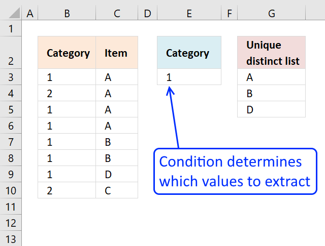
14. Create a unique distinct sorted list containing both numbers text removing blanks with a condition - Excel 365
![]()
Excel 365 formula in cell F4:
Explaining formula in cell F4
Step 1 - Compare values in column Condition to value in cell F2
The equal sign is a logical operator that lets you compare value to value, it returns a boolean value TRUE or FALSE.
Table13[Condition]=F2
and returns {TRUE; TRUE; ... ; TRUE}.
Step 2 - Check if values in column "Values" are not equal to nothing
The less than and greater than signs combined let you check if a value is not equal to another value, the result is a boolean value TRUE or FALSE.
Table13[Values]<>""
and returns {TRUE; TRUE; ... ; TRUE}.
Step 3 - Multiply arrays - AND logic
The asterisk lets you multiply numbers or boolean values in an Excel formula. Multiplying boolean values lets you perform AND logic between two values.
TRUE * TRUE = TRUE
TRUE * FALSE = FALSE
FALSE * TRUE = FALSE
FALSE * FALSE = FALSE
AND logic means that all values must be TRUE in order to return TRUE.
Also, multiplying boolean values convert them automatically to their numerical equivalents.
TRUE - 1
FALSE - 0 (zero)
(Table13[Condition]=F2)*(Table13[Values]<>"")
returns {1; 1; 0; 1; 0; 0; 0; 1; 0; 1}.
Step 4 - Filter values in Table13[Values]
The FILTER function extracts values/rows based on a condition or criteria.
Function syntax: FILTER(array, include, [if_empty])
FILTER(Table13[Values],(Table13[Condition]=F2)*(Table13[Values]<>""))
and returns {"AA"; "CC"; "DD"; 2; 2}.
Step 5 - Extract unique distinct values
The UNIQUE function returns a unique or unique distinct list.
Function syntax: UNIQUE(array,[by_col],[exactly_once])
UNIQUE(FILTER(Table13[Values],(Table13[Condition]=F2)*(Table13[Values]<>"")))
and returns {"AA"; "CC"; "DD"; 2}.
Step 6 - Sort values from A to Z
The SORT function sorts values from a cell range or array
Function syntax: SORT(array,[sort_index],[sort_order],[by_col])
SORT(UNIQUE(FILTER(Table13[Values],(Table13[Condition]=F2)*(Table13[Values]<>""))))
returns {2; "AA"; "CC"; "DD"}.
15. Create unique distinct list sorted based on text length
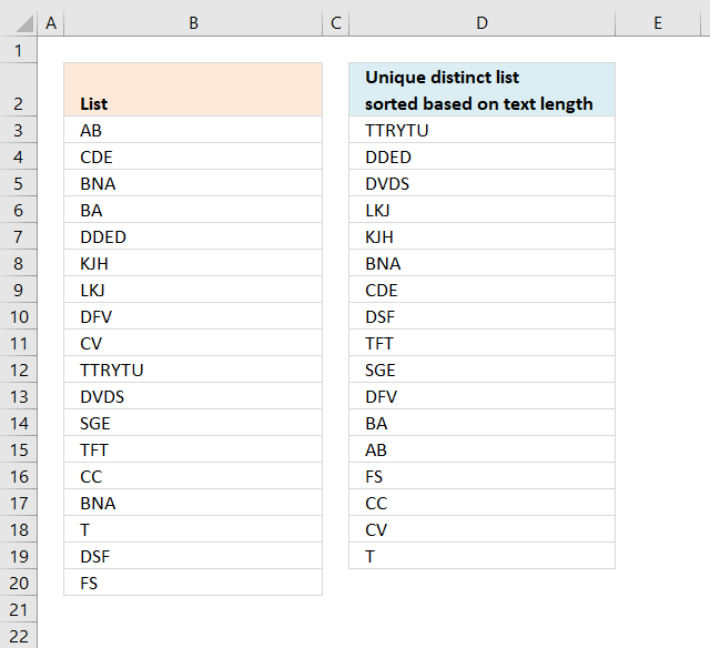
The formula in cell D3 extracts unique distinct values from B3:B20 sorted based on the number of characters, it works only with values in one column meaning your source range can't contain multiple columns.
Excel 365 formula:
Older Excel versions, array formula in D3:
To enter an array formula, type the formula in a cell then press and hold CTRL + SHIFT simultaneously, now press Enter once. Release all keys.
The formula bar now shows the formula with a beginning and ending curly bracket telling you that you entered the formula successfully. Don't enter the curly brackets yourself.
Explaining formula in cell D3
Step 1 and 2 makes sure that blanks are returned when all values have been shown.
Step 1 - Count unique distinct values
The formula returns blank values when all unique distinct values have been returned, the COUNTIF function lets you count each prior value against the list in cell range B3:B20.
COUNTIF($D$2:D2,$B$3:$B$20)
becomes
COUNTIF("Unique distinct list sorted based on text length",{"AB"; "CDE"; "BNA"; "BA"; "DDED"; "KJH"; "LKJ"; "DFV"; "CV"; "TTRYTU"; "DVDS"; "SGE"; "TFT"; "CC"; "BNA"; "T"; "DSF"; "FS"})
and returns the following array:
{0;0;0;0;0;0;0;0;0;0;0;0;0;0;0;0;0;0}
The array tells us that no value has been shown yet.
The NOT function converts TRUE to FALSE or vice versa and 1 to 0 and 0 to 1.
NOT(COUNTIF("Unique distinct list sorted based on text length",{"AB"; "CDE"; "BNA"; "BA"; "DDED"; "KJH"; "LKJ"; "DFV"; "CV"; "TTRYTU"; "DVDS"; "SGE"; "TFT"; "CC"; "BNA"; "T"; "DSF"; "FS"}))
becomes
NOT({0;0;0;0;0;0;0;0;0;0;0;0;0;0;0;0;0;0})
and returns {TRUE; TRUE; TRUE; TRUE; TRUE; TRUE; TRUE; TRUE; TRUE; TRUE; TRUE; TRUE; TRUE; TRUE; TRUE; TRUE; TRUE; TRUE}.
Then we multiply with 1 to convert the boolean values into the corresponding numerical value. TRUE -> 1 and FALSE -> 0.
{TRUE; TRUE; TRUE; TRUE; TRUE; TRUE; TRUE; TRUE; TRUE; TRUE; TRUE; TRUE; TRUE; TRUE; TRUE; TRUE; TRUE; TRUE}*1 returns {1;1;1;1;1;1;1;1;1;1;1;1;1;1;1;1;1;1}.
The SUM function adds each value in the array .
SUM({1;1;1;1;1;1;1;1;1;1;1;1;1;1;1;1;1;1})
and returns 18.
Step 2 - Compare the number to 0 (zero)
When we copy the formula and paste to cells below the cell reference expands and counts prior values. The IF function lets you decide what will happen when the logical expression returns TRUE and FALSE.
IF(SUM(NOT(COUNTIF($D$2:D2, $B$3:$B$20))*1)=0, "", formula)
becomes
IF(18=0, "", formula)
becomes
IF(FALSE, "", formula)
and returns the formula. The following steps explains the formula.
Step 3 - Count characters
The LEN function counts the number of characters in one cell, this is an array formula so the LEN function calculates the length of each value in B3:B20 and returns an array of length values.
LEN($B$3:$B$20)
returns
{2; 3; 3; 2; 4; 3; 3; 3; 2; 6; 4; 3; 3; 2; 3; 1; 3; 2}
Step 4 - Check previous values
The COUNTIF function counts values based on a condition or criteria. In this case the COUNTIF function counts previous values in order to prevent duplicate values from showing up.
COUNTIF($D$2:D2, $B$3:$B$20)
returns
{0;0;0;0;0;0;0;0;0;0;0;0;0;0;0;0;0;0}
Step 5 - Convert FALSE to TRUE
The NOT function converts boolean values, TRUE (1) to FALSE (0) and FALSE (0) to TRUE (1).
NOT(COUNTIF($D$2:D2, $B$3:$B$20))
becomes
NOT({0;0;0;0;0;0;0;0;0;0;0;0;0;0;0;0;0;0})
and returns {TRUE; TRUE; TRUE; TRUE; TRUE; TRUE; TRUE; TRUE; TRUE; TRUE; TRUE; TRUE; TRUE; TRUE; TRUE; TRUE; TRUE; TRUE}.
Step 6 - Multiply arrays
LEN($B$3:$B$20)*NOT(COUNTIF($D$2:D2, $B$3:$B$20))
becomes
{2; 3; 3; 2; 4; 3; 3; 3; 2; 6; 4; 3; 3; 2; 3; 1; 3; 2}* {TRUE; TRUE; TRUE; TRUE; TRUE; TRUE; TRUE; TRUE; TRUE; TRUE; TRUE; TRUE; TRUE; TRUE; TRUE; TRUE; TRUE; TRUE}
and returns
{2;3;3;2;4;3;3;3;2;6;4;3;3;2;3;1;3;2}.
Step 7 - Find largest value in array
The MAX function returns the largest number in the array.
MAX(LEN($B$3:$B$20)*NOT(COUNTIF($D$2:D2, $B$3:$B$20)))
becomes
MAX({2;3;3;2;4;3;3;3;2;6;4;3;3;2;3;1;3;2})
and returns 6.
Step 8 - Match the largest value to find the relative position in the array
MATCH(MAX(LEN($B$3:$B$20)*NOT(COUNTIF($D$2:D2, $B$3:$B$20))), LEN($B$3:$B$20)*NOT(COUNTIF($D$2:D2, $B$3:$B$20)), 0)
becomes
MATCH(6, LEN($B$3:$B$20)*NOT(COUNTIF($D$2:D2, $B$3:$B$20)), 0)
becomes
MAX(6, {2;3;3;2;4;3;3;3;2;6;4;3;3;2;3;1;3;2}, 0)
and returns 10.
Step 9 - Return the value from position 10.
INDEX($B$3:$B$20, MATCH(MAX(LEN($B$3:$B$20)*NOT(COUNTIF($D$2:D2, $B$3:$B$20))), LEN($B$3:$B$20)*NOT(COUNTIF($D$2:D2, $B$3:$B$20)), 0))
becomes
INDEX($B$3:$B$20, 10)
and returns TTRYTU in cell D3.
Get excel *.xlsx file
Sort text values by length_v2.xlsx
Unique distinct values category

First, let me explain the difference between unique values and unique distinct values, it is important you know the difference […]
Question: I have two ranges or lists (List1 and List2) from where I would like to extract a unique distinct […]
This article shows how to extract unique distinct values based on a condition applied to an adjacent column using formulas. […]
Excel categories
123 Responses to “Extract a unique distinct list sorted from A to Z”
Leave a Reply
How to comment
How to add a formula to your comment
<code>Insert your formula here.</code>
Convert less than and larger than signs
Use html character entities instead of less than and larger than signs.
< becomes < and > becomes >
How to add VBA code to your comment
[vb 1="vbnet" language=","]
Put your VBA code here.
[/vb]
How to add a picture to your comment:
Upload picture to postimage.org or imgur
Paste image link to your comment.
This is exactly what I've been looking for... almost. It breaks if there are blank cells in the named range. Is there a way to get this to work if there are blanks in the range?
Thanks.
Dave,
see this blog post: https://www.get-digital-help.com/extract-a-unique-distinct-list-sorted-alphabetically-removing-blanks-from-a-range-in-excel/
i cannot use an array formula for certain reasons. is there any other way?
Can you use a vba macro? Maybe someone at https://www.excelforum.com/ can help you.
Thanks sooooo much man! U Have saved my life!!!!
Great formula. With your formulas, I always modify the formula to deal with blank spaces. My data usually contains blank rows. =INDEX(List,MATCH(MIN(IF(ISBLANK(List),"",IF(COUNTIF($B$1:B1,List)=0,1,MAX((COUNTIF(List,"<"&List)+1)*2))*(COUNTIF(List,"<"&List)+1))),IF(ISBLANK(List),"",COUNTIF(List,"<"&List)+1),0). At the isblank place, you can also add other conditions like a unique list where the letter for example begins with z.
To do a descending list, change "".
This does work with numbers. Is there a way to get this to work with numbers and text?
I meant to say it does not work with numbers.
I have tried to make this work with numbers, by using an if condition to coerce a range into text -(if(isnumber(list),text(list,"0"... but I found out that countif cannot coerce a range.
Sean,
See this post: https://www.get-digital-help.com/sorting-numbers-and-text-cells-also-removing-blanks-using-array-formula-in-excel/
Oscar, Thanks. That is a great formula. Is there a way to make it so it can create a unique distinct list?
See this post: https://www.get-digital-help.com/create-a-unique-distinct-sorted-list-containing-both-numbers-text-removing-blanks-in-excel/
Thanks Oscar. This works great. For people, who want a descending sorted list, change the "" and change "+sum(" to "-sum(". This puts the numbers after the text. If you want a descending list of numbers with the numbers before the text, don't change the +sum to -sum.
Sean, isn't much easier just to use the ISTEXT function to produce the same result?
@ Oscar! Took me a whooping 3 hrs to work through the logic.... Not really gifted in this I guess! Thanks! Great formula too have for work related situations!
I was trying to use istext to convert the range into text values, but I have been told that is not possible with countif as it cannot coerce a range in memory. It would be so much easier if was able to do it that way.
[...] https://www.get-digital-help.com/create-a-unique-alphabetically-sorted-list-extracted-from... [...]
Assuming that this is more of a 'one time' type of requirement, it is also possible to achieve the desired result via:
1) Convert the numerical type of fields to actual numbers by:
a) copy any blank cell (which has a numerical value of zero) and
b) select the entire range of numbers & text cells and
c) choose
2) use the for the range ( ribbon in Excel 2007/2010)
3) sort the list
Gets the same result just without the '#N/A' whic I'm assuming is not wanted anyway.
Pat K
You can remove errors with IFERROR(value, value_if_error) function in excel 2007.
Great formula. Thanks! But it looks like it has a slight formatting mistake. Whereas you refer to the original data range as "List" almost everywhere in the formula, you have it 'hard coded' in one place. See "$A$2:$A$15" in the middle of the formula. Just replace that reference with "List".
It's amazing how many useful formulas you have here, and you're very close to what I would consider the 'ultimate' but I can't find it.
I am looking for the same formula on this page, but targeting a range of MxN (spanning multiple columns) not just a list in one column.
I see where you have formulas which act on MxN but not with all the features of this one:
1. Unique and distinct
2. Remove blanks
3. Sort
4. Properly handle numbers and text
And just to ask for the 'frosting on top' remove errors.
Thanks!
EEK,
Great formula. Thanks! But it looks like it has a slight formatting mistake. Whereas you refer to the original data range as "List" almost everywhere in the formula, you have it 'hard coded' in one place. See "$A$2:$A$15" in the middle of the formula. Just replace that reference with "List".
Thanks, I have edited this post.
EEK,
read this post: Excel 2007/2010 array formula: Filter unique distinct values, sorted and blanks removed
Great piece of art.
I have a question here:
Assuming the range List is in B19:B39
Shortened list is in C80:C85
How can this formula be amended to show correct values?
ahmed,
Instructions:
1. Create a named range (named List) and use cell range B19:B39
2. Select cell C80 and type in formula bar:
=INDEX(List, MATCH(MIN(IF(ISBLANK(List)+COUNTIF(C79:$C$79, List), "", IF(ISNUMBER(List), COUNTIF(List, "<"&List), COUNTIF(List, "<"&List)+SUM(IF(ISNUMBER(List), 1, 0))+1))), IF(ISBLANK(List)+COUNTIF(C79:$C$79, List), "", IF(ISNUMBER(List), COUNTIF(List, "<"&List), COUNTIF(List, "<"&List)+SUM(IF(ISNUMBER(List), 1, 0))+1)), 0)) 3. Press and hold Ctrl + Shift 4. Press Enter once 5. Release all keys. Copy formula 1. Select cell C80 2. Copy (Ctrl + c) 3. Select cell range C81:C85 4. Paste (Ctrl + v)
Hi Oscar,
Thanks for these amazing formulas. If the numbers in the list include single and double digit numbers and I need the list to be ordered correctly i.e. 1-9 10-100 and then text. Currently the formula produces 1,10,11,12etc and then 2,20,21 etc.
Apologies, I did not complete the question. Basically is it possible to adapt the above to create the list in the correct order?
Harry,
Is this the problem?
I don´t know how to solve that, sorry.
Hi Oscar,
The problem is not quite as you say but very similar. The list being used in the formula changes dynamically based on a choice made elsewhere on the spreadsheet. This master list is either text or a list of numbers which are read as text. I fixed my problem for now by adding a 0 before any number which is less than 10. This means I do not need to sort the data as it now comes into my sheet corted correctly.
For those people searching through this and have a very long master list that needs to be compacted into a much shorter unique list I found that your formula can take a while to calculate and slows the sheet down. I was keen to avoid macros whilst building the s/s but the following macro works quite well and is relatively easy to adapt.
Sub RF_list()
With Sheets("Master")
.Range(.Range("F2"), .Range("F65536").End(xlUp)).Copy
End With
Sheets("Tables").[H3].PasteSpecial Paste:=xlValues
ActiveSheet.Range("$H$3:$H$10000").RemoveDuplicates Columns:=1, Header:=xlNo
ActiveWorkbook.Worksheets("Tables").Sort.SortFields.Clear
ActiveWorkbook.Worksheets("Tables").Sort.SortFields.Add Key:=Range("H3"), _
SortOn:=xlSortOnValues, Order:=xlAscending, DataOption:= _
xlSortTextAsNumbers
With ActiveWorkbook.Worksheets("Tables").Sort
.SetRange Range("H3:H899")
.Header = xlNo
.MatchCase = False
.Orientation = xlTopToBottom
.SortMethod = xlPinYin
.Apply
End With
End Sub
Hope this helps someone out there.
Regards
Harry
Sean, awesome stuff. In one of the first comments you state " For people, who want a descending sorted list, change the "" and change "+sum(" to "-sum(". This puts the numbers after the text. If you want a descending list of numbers with the numbers before the text, don't change the +sum to -sum."
I would like to have the numbers descending followed by the text. You note indicates I should change the "" and leave everything else. However, you don't indicate what I should change the "" to. Thank you for your help. I am using the following formula as base:
IFERROR(=INDEX(List, MATCH(MIN(IF(ISBLANK(List)+COUNTIF(B1:$B$1, List), "", IF(ISNUMBER(List), COUNTIF(List, "<"&List), COUNTIF(List, "<"&List)+SUM(IF(ISNUMBER(List), 1, 0))+1))), IF(ISBLANK(List)+COUNTIF(B1:$B$1, List), "", IF(ISNUMBER(List), COUNTIF(List, "<"&List), COUNTIF(List, "<"&List)+SUM(IF(ISNUMBER(List), 1, 0))+1)), 0)), "")
Thanks for the formula. How do I extend it beyond 10 lines?
If I copy the formula from B2 and Ctrl+Shift+Enter it into B11, B12 etc. I just see "BB" repeated.
--Thanks.
Jay,
Copy the cell, not the formula.
The formula contains relative cell references that change when you copy the cell.
Oscar.
I am using the formula for creating the list with criteria and I am running into a problem. My data is on a different sheet to where I am using the formula and I have referenced the cell 'name' and 'task'. I want to create a list of names based on the task they are doing. I have copied the formula and have entered it as an array and it has the { } brackets around it. All I am getting is one name repeated down the list. I'm not sure where I am going wrong.
Thanks, Ollie.
Ollie Wood,
I think you found the answer above. Copy the cell, not the formula.
Here it is again in greater detail:
1. Select the cell
2. Copy cell (Ctrl + c)
3. Select the cell range below.
4. Paste (Ctrl + v)
The formula contains relative cell references that change when you copy the cell.
Oscar
Thanks for the quick reply. I had read this and this is how I am coping it, using ctr c and v. It's still not right though. Can you offer any other pointers where I may be going wrong?
Thanks, Ollie.
Ollie Wood,
Send me your workbook (without sensitive data):
Contact form
Hi Ollie, I had the same problem, you have to remove any blank cells from the list, or use the modified version of the formula that deals with blanks.
Oscar is it possible to add something to the sample sheet so the formula ignores blank cells? I've tried adapting it myself but with no luck.
Rob,
Read this post:
Create a unique distinct sorted list containing both numbers text removing blanks
Hello, Oscar!
It is exciting material to me, I thought of something like that before but was not able to invent it.
But I cannot understand it. :(
For example - why are we making Max of CountIf result? As CountIf result should be a single value, than Max of it is going to be the same value isn't it?
Alexander,
why are we making Max of CountIf result? As CountIf result should be a single value, than Max of it is going to be the same value isn't it?
No, The countif function returns an array of values.
Get the Excel the attached file and "Evaluate" the formula.
Wow interesting tool, thanks you! You opened me eyes!
The only issue "Evaluate" have is its unusable window - it doesn't format formula in any way, it dosn't allow copy, it doesn't allow resize.
In general it is just magic, thanks.
If you have time and will to answer -
Why
ROW(List)
works differently when I bring it out of the whole formula?
ROW(List) always return me row of the list start not the corresponding item's row.
Alexander
List is named range, example A1:A10.
Example 1,
Array formula: =ROW(List)
returns {1; 2; 3; 4; 5; 6; 7; 8; 9; 10} but only 1 is visible in the cell.
Example 2,
Array formula: =IF(ROW(List)=1,1,0)
becomes
=IF({1; 2; 3; 4; 5; 6; 7; 8; 9; 10}=1,1,0)
becomes
=IF({TRUE; FALSE; FALSE; FALSE; FALSE; FALSE; FALSE; FALSE; FALSE; FALSE},1,0)
and returns {1; 0; 0; 0; 0; 0; 0; 0; 0; 0}
but only the first value in the array is visible. A single cell can´t display all values in an array.
Thank you, very intresting!
Hope I don't mess here too much.
Wanted to ask - where did you learn excel that good from? May you suggest some good book or web resource.
As for me - I like Excel, use it where possible, but I'm not even close.
Hi Oscar,
Thank you so much for your very helpful posts - I look forward to receiving each one and find them very educational and useful.
I have a question about hyperlinks. I have a main table (which holds all my income and spend information) and I scan every receipt and put a hyperlink on the supplier of items I purchase which enables me to call up the receipt (which I save in pdf format).
I have built sheets using array formulas that query the main table based on dropdown boxes to identify record numbers meeting whatever criterion I want, and then display details of the records (using a simple offset function against the record number). However, to see any receipts, I have to go back to the main table and find the original entry to access the hyperlink.
Is there any way to display the hyperlink along with the other information I pull from the master table, so that I can access the receipts from the query sheet?
Thanks so much for your help.
Regards
Geoff Robb,
Save your receipt´s filepaths and file names in a column on your main table. I believe you can query and insert that data in your hyperlink formula on your query sheet.
Oscar,
Great work on the excellent posts. They are very helpful.
I am trying to use an adaptation of this idea, but am not able to get the formula working. In the first column I have a list that should be unique but may be unsorted. In the second column I have a Yes/No value to choose whether or not to include that row in the final result list. The final result list should be sorted. Is this possible?
For example:
List Include
AA Yes
CC Yes
BB No
DD Yes
EE No
Final result list:
AA
CC
DD
Thanks for your help!
Regards
Glen,
Array formula in cell G2:
=INDEX($D$2:$D$7, MATCH(MIN(IF((COUNTIF($G$1:G1, $D$2:$D$7)=0)*($E$2:$E$7="Yes"), 1, MAX((COUNTIF($D$2:$D$7, "<"&$D$2:$D$7)+1)*2))*(COUNTIF($D$2:$D$7, "<"&$D$2:$D$7)+1)), COUNTIF($D$2:$D$7, "<"&$D$2:$D$7)+1, 0)) Get the Excel *.xls file unique-list-sorted-alphabetically-with-a-condition.xls
Excellent, that works like a charm. Well, almost... It turns out that the list could contain both text and numbers. If the list contains a number, this formula no longer works correctly.
I saw your separate post about sorting text and numbers https://www.get-digital-help.com/sorting-numbers-and-text-cells-also-removing-blanks-using-array-formula-in-excel/ but it is not clear to me how to add the condition *($E$2:$E$7="Yes") to it.
As before, any guidance is greatly appreciated!
Glen,
read this post: Create a unique distinct sorted list containing both numbers text removing blanks with a condition
Brilliant, Oscar! That works perfectly.
Thanks for the help.
Why won't this work for a named range that is on another sheet? Sorry, newbie here.
Lauren,
If you are talking about this formula:
=INDEX(List, MATCH(MIN(IF(COUNTIF($B$1:B1, List)=0, 1, MAX((COUNTIF(List, "<"&List)+1)*2))*(COUNTIF(List, "<"&List)+1)), COUNTIF(List, "<"&List)+1, 0)) I does work but you have to enter it as an array formula. 1. Select a cell 2. Press with left mouse button on formula bar 3. Copy and Paste array formula in formula bar 4. Press and hold Ctrl + Shift 5. Press Enter
Hi Oscar!
Can you help me?
I have a name products column and their prices (other column).
I want to create unique distinct list with products name sorted by SUM of prices. Is it real using array formula?
Bill,
read this post:
Filter unique distinct list sorted based on sum of adjacent values
Thanks, Oscar!
great, but keep getting a #NUM! error after cell b2
any reaason this would calculate REALLY slowly?
brendan,
Array formulas working with large data sets can be slow. It also depends on your computer hardware.
Hi Oscar, Great Formula!!
Just wondering, how can the original formula you used in the article be further expanded to account for a criteria. I'll explain further.
Using your example,
Column A Column B
List Weight
DD 1
EE 0
FF 0
EE 1
GG 0
BB 1
FF 1
GG 0
DD 1
DD 0
FF 1
AA 0
EE 0
How can I then create a unique list of Column A - say in column D - for those with 0 in column B, and then another unique (i.e. no repition of AA, BB) list of Column A - say in column E - for those with 1 in column B?
I've tried to manipulate the original formula you created, but failed. Would greatly appreciate your help. :)
Thanks :)
Peter
Peter,
read this:
Create a unique distinct alphabetically sorted list with criteria
Thanks. Perfect!!
Actually, I have a further idea, Say we had a third weight (say 2) and we now wanted a list of 1 and 0 together as one list, and 2 as a separate list. How would the formula be then? Because:
(...) *($B$2:$B$14=1)*($B$2:$B$14=0)* (...) Wouldn't work.
Thanks
Peter
Peter,
Array formula in cell D6:
=INDEX($A$2:$A$16, MATCH(MIN(IF((COUNTIF($D$5:D5, $A$2:$A$16)=0)*(COUNTIF($D$2:$D$3,$B$2:$B$16)), 1, MAX((COUNTIF($A$2:$A$16, "<"&$A$2:$A$16)+1)*2))*(COUNTIF($A$2:$A$16, "<"&$A$2:$A$16)+1)), IF(COUNTIF($D$2:$D$3,$B$2:$B$16), COUNTIF($A$2:$A$16, "<"&$A$2:$A$16)+1,""), 0)) Array formula in cell E6: =INDEX($A$2:$A$16, MATCH(MIN(IF((COUNTIF($E$5:E5, $A$2:$A$16)=0)*(COUNTIF($E$2,$B$2:$B$16)), 1, MAX((COUNTIF($A$2:$A$16, "<"&$A$2:$A$16)+1)*2))*(COUNTIF($A$2:$A$16, "<"&$A$2:$A$16)+1)), IF(COUNTIF($E$2,$B$2:$B$16),COUNTIF($A$2:$A$16, "<"&$A$2:$A$16)+1,""), 0)) Get the Excel *.xlsx file Create-a-unique-distinct-alphabetically-sorted-list-with-criteria-v2.xlsx
Hi Oscar,
I am trying to use the formula for the list in Column C and paste at column G. Changing that in the formula is not helping.
Could you please help.
Sorry, found exactly where I was going wrong.
[...] https://www.get-digital-help.com/create-a-unique-alphabetically-sorted-list-extracted-from... [...]
[...] Look here: Create a unique distinct alphabetically sorted list, extracted from a column in excel | Get Digital ... [...]
I am using the following formula. How can i get it to work if there are blank cells?
How can i get it to work if there are formulas in the column?
=IFERROR(INDEX(List1,MATCH(MIN(IF(COUNTIF($F$9:F9,List1)=0,1,MAX((COUNTIF(List1,"<"&List1)+1)*2))*(COUNTIF(List1,"<"&List1)+1)),COUNTIF(List1,"<"&List1)+1,0)),"")
Jimmie,
try this formula:
=INDEX(List, MATCH(MIN(IF((List="")+COUNTIF(B1:$B$1, List), "", IF(ISNUMBER(List), COUNTIF(List, "<"&List), COUNTIF(List, "<"&List)+SUM(IF(ISNUMBER($A$2:$A$15), 1, 0))+1))), IF((List="")+COUNTIF(B1:$B$1, List), "", IF(ISNUMBER(List), COUNTIF(List, "<"&List), COUNTIF(List, "<"&List)+SUM(IF(ISNUMBER(List), 1, 0))+1)), 0)) Get the Excel file Unique-and-Sort-numbers-and-text-cells-using-excel-array-formula-works-with-formulas.xls
I was trying to use your technique, could I use an entire column instead of a Range? Range is fine actually I tried to rename it Destinations, but my real problem maybe I want the Range to be on Worksheet and the summary of unique values, they don't even need to be sorted on another Worksheet. I get a N/A when I try it. I try modifying the formual to start in Column A in cell 2 when making the list, the attached example works so I may peck away at that.
Suggestions?
Hi
I'm getting a problem when i using your formula in two different sheet. Although its working in the single sheet.
On same sheet reference.
+ CTRL + SHIFT + ENTER
I'm using this on different sheet reference.
+ CTRL + SHIFT + ENTER
Plz correct my formula.
Abhinav,
Try this formula on the other sheet:
That worked like a charm... :)
Thanks so much Oscar...!!!
Personally, I use the Google spreadsheets all the time for uniques, sorting, filtering and queries. It's so much better than Excel for that.
The simplest method in Excel is to
Highlight a range of data (make sure they all have a heading)
Go to Insert tab
Select Pivot Table
Choose new or existing worksheet, your choice
Press with left mouse button on OK
In the PivotTable Field List find your column you want to sort
Drag that into the Row box at the bottom
You can now sort the list alphabetically if you want from the Row Labels Filter button.
You can go to Pivot Table options to remove headings, sorting options, auto width, subtotals and other stuff.
That's it.
VisicalcVeteran,
Personally, I use the Google spreadsheets all the time for uniques, sorting, filtering and queries. It's so much better than Excel for that.
Competition is great!
The simplest method in Excel is to
Highlight a range of data (make sure they all have a heading)
Go to Insert tab
Select Pivot Table
Choose new or existing worksheet, your choice
Press with left mouse button on OK
In the PivotTable Field List find your column you want to sort
Drag that into the Row box at the bottom
You can now sort the list alphabetically if you want from the Row Labels Filter button.
You can go to Pivot Table options to remove headings, sorting options, auto width, subtotals and other stuff.
That's it.
A lot of steps if you have to repeat it many times.
An array formula and a named range is a lot quicker, in my opinion.
Hi Oscar, have been reading your blog over the last few weeks and have learnt a bunch of new techniques as a result.
I have been working with one of the unique list array formulas and it works a treat. I was wondering however if it is possible to add a criteria outside the array to effectively filter the list by a further level? The formula I have is
=IFERROR(INDEX(STATSUBCAT, MATCH(MIN(IF(ISBLANK(STATSUBCAT)+COUNTIF(D7:$D$7, STATSUBCAT), "", IF(ISNUMBER(STATSUBCAT), COUNTIF(STATSUBCAT, "<"&STATSUBCAT), COUNTIF(STATSUBCAT, "<"&STATSUBCAT)+SUM(IF(ISNUMBER(STATSUBCAT), 1, 0))+1))), IF(ISBLANK(STATSUBCAT)+COUNTIF(D7:$D$7, STATSUBCAT), "", IF(ISNUMBER(STATSUBCAT), COUNTIF(STATSUBCAT, "<"&STATSUBCAT), COUNTIF(STATSUBCAT, "<"&STATSUBCAT)+SUM(IF(ISNUMBER(STATSUBCAT), 1, 0))+1)), 0)),"")
I'm working (as a learning process!) on a personal budget spreadsheet. Using bank statements and the adding a column to categorize the transactions then SUMIF in the adjacent column I have a helpful look into my total catergory spending.
At the moment I am getting what the array formula is supposed to do; provide a list of all unique category types. But say I wanted to see what categories appeared between 2 dates? I tried adding a simple IF statement into the array formula just to select one date to see if I could get any matches to return. It did not so I guess I'm inserting the statement at the wrong position assuming this is possible at all?
Thanks again for a taking the time to put together such an instructive site.
To save anyone looking into this I should say I had my problem on its head. I had all I needed all along and simply needed to add a SUMIFS formula to filter the original data.
Just confirms stepping away from a problem for an hour or so is often the best thing you can do.
Duncan,
Yes, you can use sumifs. Have you tried a pivot tables?
https://chandoo.org/wp/2009/08/19/excel-pivot-tables-tutorial/
https://www.contextures.com/CreatePivotTable.html
Hi Oscar,
I'm thinking pivot tables will have to be on my to learn list but for now it's info overload and I'm still getting to grips with some of the other stuff first. Also I have an awful lot of catergories in my Unique list that certainly benefit in terms of screen real estate from just displaying the ones needed to display the results.
To which end can could you help me abbreviate the formula so that it is only concerned with text entries and blanks (I'm only using the formula to create the unique category and subcategory expense description). I've noticed as this workbook is developing the CPU usage is starting to get out of hand on this moderate i3 3.2ghz machine. I'd rather not have to resort to manual calculation if I can help it.
I've stripped all the volatile date filtering out, TODAY() etc and that doesn't appear to be the source of the high CPU call?
I keep breaking the formula when I have tried to strip out the number functions, I hopefully as I get more familiar with the syntax I'll be able to say I have a better degree of understanding of how all the parts sit together.
Best,
Doh! Sorry Oscar were you suggesting I keep the Array for the Unique value then use those as row labels for the different column headers?
The jpg attached is an early draft and so far I've only SUMIFS the date ranges for the main expense catergory, the next block is the subcatergory to the right will hopefully receive the same treatment CPU overhead allowing.
Can I employ a Pivot table when the Catergory descriptions may change. I suppose in time all catergories will appear but that said I am really liking the idea of this unique array deal.
If you think its possible I'll be happy to go off and do the proper researh
Thanks again
Duncan,
Pivot tables lets you create unique values and sum corresponding values. It is really easy.
You can also filter the data using dates.
Oscar,
How right you were. What a revelation!
Took me a while to spot the Group.. function to assist in gathering my Date column headers into months but once I did I now have everything I need and at hardly any CPU cost.
I am now looking at the multiple consolidation ranges to see if this will allow me to get the necessary summary overview of all account pivot tables.
Thanks again..
Yo!
Very good formula you have here, but very complicated and useful for few list only (hang on 500+ data). I have here my own and simple way, yet effective. I been using this for 3 years. Using only countif, vlookup and rank.
DATA is on Column C.
Formula to get unique values is on Column B
Formula to sort the unique values on Column A
The unique list in on column D.
A2=if($b2="zzz","",countif($b$2:$b$6,"<="&$b2))
B2=if(countif($c$1:$c2,$c2)=1,$c2,"zzz")
D2=iferror(vlookup(rows($d$2:$d2),$a:$c,2,0),"")
Row Column A Column B Column C Column D
1 Sort get Unique Data Unique list
2 2 mark mark ann
3 zzz mark mark
4 3 zack zack zack
5 1 ann ann
6 zzz zack
Hope this helps you as it did to me. I been using this to my 10,000 rows of name and get the sorted unique names.
mark
Awesome, thx! The issue with the solution proposed above - as you stated - is that it doesn't work for large tables (that's why the commenter above was seeing the same value in all rows, it wasn't a copy/paste issue, just slow calcuation). This is less elegant but more effective. Thanks!
[…] Here is a possible solution. I found this amazing formula for unique values online at Create a unique distinct alphabetically sorted list, extracted from a column in excel | Get Digital … Note that the formula uses a few named ranges for simplicity, make sure you add those, If you want […]
Hi, It is amazing formual and it is working. However, despite trying hard, I fail to understand what the MATCH formula exactly doing in this. I am newbie for such complicated formulas.
So, Please explain in workds what following formula is doing.
Is there a way to do this without it being a array formula?
john dalton,
Perhaps there is, try this:
https://www.get-digital-help.com/no-more-array-formulas/
[…] at Create a unique distinct alphabetically sorted list, extracted from a column in excel | Get Digital … or filter -> advanced filter -> unique […]
Hello,
I've tried the V2 formula, and it works well. But, apparently it'll make a blank result too if i make a blank list in the column A. I wanna skip the blank list without breaking the formula logic, can anyone resolve this? Thanx.
Oscar,
I need to sort from largest value to smallest and continue to have issues. I'm working with values and have flipped SMALL to LARGE and Min to MAX. I must be missing something simple, could you please point me in the correct direction?.
Appreciate all the help.
Alex
wow man, u blew me away.. i've been looking for this for a long time. ur algorithm is bright. Ive tried PIVOT TABLE but it wont update if u copy it, ADVANCED FILTER but u have to do it over and over. im using a multiple table report and this what im trying to create but no luck. u did great bro.. ive search about circular references coz i know that would do it but its too complex for my level.. thanks bro. ur the man!!!
[…] I can summarize my product data with a sumifs statement. I can get unique customer data from multiple from the method described here: unique distinct value […]
How about "Z to A"?
Thanks lots!
Great formula! You guys are amazing and I appreciate what you do. I'm having one particular issue with the formula.
I want to reference the unique values created by this formula, in order to calculate other values in my workbook. The issue I'm having is that every time excel calculates, the unique list changes.
For example, here is one unique list:
A1B
A1B*UP
A1F
A1F*UP
When I press F9 to calculate, I get the following (probably due to the sorting)
A1B*UP
A1B
A1F*UP
A1F
Is there any way to have it so that the unique values sort consistently one way or the other?
Thanks!
Hello,
In your 'Create a unique distinct alphabetically sorted list with criteria' which is fantastic by the way, I need to extend this to have a third column 'c' with its own criteria and a column 'f' which lists those indicated in 'c'.
To clarify:
column 'e' would be a sorted list from 'a' depending on 'b'
column 'f' would be a sorted list from 'a' depending on 'c'
Try as I might, I cannot seem to get the formula correct to do this, your help would be really appreciated.
Thank you
Tony
Hello,
Congratulations. The formula is amazing.
The "Create a unique distinct sorted list containing both numbers text removing blanks with a condition" example is almost perfect for me.
But I´d like to remove the DISTINCT condition.
Could you please help me?
Regards
Whenever I use this I keep getting a blank in the second row for the created list.
Other than that it is working fine. I just don't understand what would cause that.
Thanks! It worked for me. I used this to remove blank spaces from a total of 2520 entries.
If it is an option, I have gotten in the habit of using this formula:
=IFERROR(INDEX(A:A,MATCH(0,INDEX(COUNTIF($B$1:B3,A:A),0,0),0)),)
And simply starting in B4 with B1=BLANK B2=0 and B3="Header"
That way it reads blanks and 0s as non-unique values in the list, and they are ignored. I will then hide rows 1:2.
The formula looks for values in the range (A:A in the example) not previously occurring in the list above the current cell ($B1:$B3 in the example). B4 examines $B$1:$B3, B5 examines $B$1:$B4 and so on.
Perhaps not the most elegant way, but it gets the job done and does not require arrays or more complex formulae.
Nice Formula/Solution!
Hi, the formula only works if I paste it into cell B2. If I try to change the formula cell reference from B1 to the cell that I need (cell C33), it returns an #N/A error. Do you have any advice? Thanks.
Great Formula!
What if I want to create a unique distinct sorted list containing both numbers and text, removing blanks with 2 or more conditions?
Thanks,
Brett
Is there a way to apply this to a filtered range and have it ignore hidden values? I'm using this formula and it works really well, but it shows every unique value in my range (R12:R1200) including the hidden ones. Any ideas?
=INDEX($R$12:$R$1200, MATCH(0, IF(ISBLANK($R$12:$R$1200), 1, COUNTIF(Z2:$Z$2, $R$12:$R$1200)), 0))
Hi Rod,
Yes, there is.
https://www.get-digital-help.com/extract-unique-distinct-values-from-a-filtered-table-udf-and-array-formula/
Thank you, Oscar! That worked! I'll rely to that post with a related question.
Great series of blogs Oscar. I think i almost have what I need. I'm struggling to get my list sorted alphabetically (it has a date filter and some key word filters in it already). I'm probably getting confused by all the syntax. Any chance of some tips?
Start Date B1
End Date B2
{=IFERROR(INDEX(TblDelivery, MATCH(0,IF(LEFT(TblDelivery[Product],3)="PRO",1,COUNTIF($B$5:$B5,TblDelivery[Product])+(TblDelivery[Date]>$B$2)+(TblDelivery[Date]<$B$1)),0),COLUMN(E1)),"")}
Thanks
Adrian
Adrian
This might work:
=INDEX(TblDelivery[Product], MATCH(MIN(IF((COUNTIF($B$5:$B5, TblDelivery[Product])=0)*(TblDelivery[Date]>$B$2)*(TblDelivery[Date]<$B$1), 1, MAX((COUNTIF(TblDelivery[Product], "<"&TblDelivery[Product])+1)*2))*(COUNTIF(TblDelivery[Product], "<"&TblDelivery[Product])+1)), IF((TblDelivery[Date]>$B$2)*(TblDelivery[Date]<$B$1),COUNTIF(TblDelivery[Product], "<"&TblDelivery[Product])+1,""), 0))
Hi,
I'm just applying the LEFT() function on 'list' as
left(list,2), I'm getting error as
"There's a problem with this formula.
you type: =1+1, cell shows: 2"
Any help regarding this?
Qadeer Ahmed
You need to create a named range.
1. Select the cell range you want to use.
2. Press with left mouse button in the name box (next to the formula bar) and name the range. In this case, list.
3. Press Enter
Thank You!
This formula doesn't work for at all - I either get an entire list of n/a, or a value that doesn't even exist on my list!
I have a column of dates: I just want another column to show me a list of all unique dates in the first column.
Joy
You need to adjust the cell references in the formula so they point to your data:
=LOOKUP(2, 1/((COUNTIF($D$2:D2, $B$3:$B$12)=0)*($B$3:$B$12<>"")), $B$3:$B$12)
Cell reference $D$2:D2 is different, if you enter the formula in cell G5 the cell reference becomes $G$4:G4. meaning it should always be a cell reference to the adjacent cell right above.
You then copy the cell and paste it to cells below as far as needed, this will automatically change the relative cell references in the formula.
Hey! So Excel has a "UNIQUE" function now. Do you please have any ideas on how to extract them from that function?
Andrew,
yes, use the FILTER function to exclude blank cells.
=UNIQUE(FILTER(B3:B12,B3:B12<>""))
Hello Oscar,
Great and very helpful website!
I am looking to return a unique list across multiple columns and rows. I had assumed I could just expand
$B$3:$B$12to my criteria$A$5:$G$30but this just seems to return #N/AIs there a way of obtaining a unique list based from multiple columns and rows?
What I am ultimately looking to do is list them in the order of most frequent result at the top
Ollie,
Is there a way of obtaining a unique list based from multiple columns and rows with most frequent result at the top?
Yes, there is. Read this:
Extract a unique distinct list across multiple columns and rows sorted based on frequency
Have been using the UDF to great effect but I have been asked if there is a way to add a list of other items to exclude along with the blanks
I know I can modify the line -
If Len(Value) > 0 Then ucoll.Add Value, CStr(Value) to include
If Len(Value) > 0 And Value "Cancelled" And Value "N/A" Then ucoll.Add Value, CStr(Value)
but this is rather inelegant there must be a way to add an array or list to the top of the UDF which would be easier to manage but my VBA is a little to rusty to figure it out
Hi Oscar,
This doesn't work for a range across multiple columns. Do you know if it's a small adjustment to the formula to allow this or will it only work for a single column?
Kristo,
those formulas above work only for a single column, the following Excel 365 formula works with a multi-column cell range:
This formula works with many multicolumn cell ranges