How to use the FILTER function

The FILTER function lets you extract values/rows based on a condition or criteria. It is in the Lookup and reference category and is only available to Excel 365 subscribers.
What's on this page
- Syntax
- Example
- Filter values based on a condition
- Why does the FILTER function return a #NAME? error?
- Is the FILTER function available for Excel versions 2003, 2007, 2010, 2013, 2016, and 2019?
- The FILTER function returns a #SPILL! error, why?
- Why does the FILTER function return a #CALC! error?
- Can I use the FILTER function with an Excel Table and structured references?
- Can the FILTER function handle error values?
- Is the FILTER function case sensitive?
- based on a condition - case sensitive
- If not equal to
- If smaller than
- If larger than
- If contains
- If not contain
- Begin with
- End with
- Based on a condition sorted from A to Z
- Based on criteria
- Based on a condition per column - AND logic
- Based on a condition per column - OR logic
- #CALC! error returns [if_empty] argument
- Get Excel file
- Lookup and return multiple sorted values based on corresponding values in another column - Excel 365
- Lookup and return multiple sorted values based on corresponding values in another column - previous Excel versions
- Lookup and return multiple sorted values based on corresponding values in another column - Excel Table
- Function not working
1. Syntax
FILTER(array, include, [if_empty])
| Argument | Text |
| array | Required. Cell range or array. |
| include | Required. An array containing True or False that match the rows and columns of the array argument. |
| [if_empty] | Optional. The FILTER function returns #CALC! if the result is empty. [if_empty] is a value you define to avoid the #CALC! error. |
3. Example
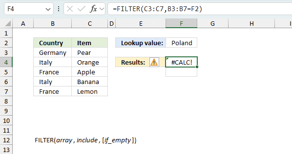
The image above shows a regular formula in cell D3:
The formula above filters the data set in cell range C3:C7 based on the condition specified in cell F2. The output is an array and is returned to cell F4 and cells below as far as needed.
4. Filter values based on a condition
The Filter function filters values in cell range C3:C7 if a value in B3:B7 on the corresponding row equals "France" (Cell F2).
Formula in cell D3:
There is a formula for you that have an earlier Excel version than Excel 365: VLOOKUP - Return multiple values [vertically]
The FILTER function has three arguments, the second one is an array that evaluates to TRUE or FALSE or their numerical equivalents 1 or 0 (zero).
FILTER(array, include, [if_empty])
B3:B7=F2
The equal sign is a logical operator that evaluates if cell values in B3:B7 are equal to cell value in F2, one by one.
B3:B7=F2
returns {FALSE; FALSE; TRUE; FALSE; TRUE}.

The image above shows the array in column A, the values correspond to the values in column B, True is on the same row as France row 5 and 7. False is on all remaining rows.
The FILTER function uses this array containing boolean values (TRUE or False) to determine which values to return from column C. "Apple" and "Lemon" are on the same row as France row 5 and 7. The values are returned to cell F4 and cells below if needed.
The FILTER function may return an array and Microsoft calls this a dynamic array meaning the values are automatically entered to cells below without the need for an array formula.
1.1 Why does the function return a #NAME? error?
First, make sure you correctly spelled the FILTER function. If the FILTER function still returns a #NAME? error you probably use an earlier Excel version and can't the FILTER function unless you upgrade to Excel 365.
There is a small formula you can use if you don't have access to the FILTER function, check it out here: VLOOKUP - Return multiple values [vertically]
1.2 Is the function available for Excel versions 2003, 2007, 2010, 2013, 2016, and 2019?
No, only Excel 365 subscribers have it. However, I made a small formula that works fine, check it out here: VLOOKUP - Return multiple values [vertically]
1.3 The function returns a #SPILL! error, why?
The FILTER function returns an array of values and tries to automatically use the appropriate cell range needed to show all values. If one or more cells are occupied with other values the FILTER function returns #SPILL! error.
You have two options, delete or move the values that cause the error or deploy the FILTER function in another cell that has empty cells below.
1.4 Why does the function return a #CALC! error?
The FILTER function returns a #CALC! error if the output result has no values, make sure you enter the third argument to define a value if dynamic array is empty, to avoid the #CALC! error.
1.5 Can I use the function with an Excel Table and structured references?
Yes, you can. The FILTER function recalculates the output automatically if you add, edit or delete values in the Excel Table.
1.6 Can the function handle error values?
No, the FILTER function stops working if there are error values in the second argument. An error in the first argument is passed on to the output array with other regular values.
1.7 Is the function case sensitive?
No, the FILTER function is not case sensitive if you use the equal sign. Read the next section for how to make the FILTER function case sensitive.
5. Extract values based on a condition - case sensitive

The image above shows a formula in cell F4 that extracts values from column C if the corresponding values in column B match the value in cell F2.
There is a formula for you that have an earlier Excel version than Excel 365: Case sensitive lookup and return multiple values
The EXACT function returns True if both arguments are exactly the same considering upper and lower letters as well.
EXACT(text1, text2)
The EXACT function allows you to use a cell range in the first argument and the result is an array that matches the size of the first argument as long as the second argument is a single value.
EXACT(B3:B7,F2)
returns {TRUE; FALSE; FALSE; FALSE; TRUE}.
FILTER(C3:C7,EXACT(B3:B7,F2))
returns {"Pear"; "Lemon"} in cell range F4:F5.
6. Extract values if not equal to

The image above demonstrates the FILTER function in cell F4, it returns all values from column C if the corresponding values in column B are not equal to the value in cell F2.
The less than and larger than characters combined means "not equal to".
B3:B7<>F2
returns {TRUE; TRUE; FALSE; TRUE; FALSE}.
FILTER(C3:C7,B3:B7<>F2)
returns {"Pear"; "Orange"; "Banana"} in cell range F4:F6.
7. Filter values smaller than a condition

The image above shows a formula in cell F4 that extracts values from column B if the corresponding value in column C is less than the number in cell F2.
The less than character < is a logical operator that checks if a number is smaller than another number. In this demonstration, we will apply this to a cell range C3:C7. The logical expression is:
C3:C7<F2
returns {FALSE; TRUE; FALSE; TRUE; TRUE}.
FILTER(B3:B7, C3:C7<F2)
returns {"Orange"; "Banana"; "Lemon"}.
8. Extract values if larger than the given condition

Formula in cell F4:
The larger than character > is a logical operator that evaluates to True if a number is larger than another number otherwise False. In this demonstration, we will apply this to a cell range C3:C7. The logical expression is:
C3:C7>F2
becomes
{6;2;7;3;2}>5
and returns {TRUE; FALSE; TRUE; FALSE; FALSE}.
FILTER(B3:B7, C3:C7>F2)
becomes
FILTER({"Pear";"Orange";"Apple";"Banana";"Lemon"}, {TRUE; FALSE; TRUE; FALSE; FALSE})
and returns {"Pear"; "Apple"}.
9. Extract values if cell contains given string

The image above shows a formula in cell F4 that extracts values from column C if the corresponding value in column B contains the given string in cell F2.
Formula in cell F4:
The formula in cell F4 returns "Pear", "Apple" and "Lemon" because the corresponding values in column B "Germany", "France" and "France" contain string "r".
Step 1 - Identify cells containing string
The SEARCH function has these arguments: SEARCH(find_text,within_text, [start_num])
It returns a number representing the character position of the found string, an error is returned if not found. The SEARCH function does not perform a case sensitive search, use the FIND function for that.
SEARCH(F2,B3:B7))
returns {3; #VALUE!; 2; #VALUE!; 2}.
Step 2 - Replace errors
The FILTER function can't handle errors in the second argument include. FILTER(array, include, [if_empty])
ISNUMBER(SEARCH(F2,B3:B7))
returns {TRUE; FALSE; TRUE; FALSE; TRUE}.
Step 3 - Filter array
FILTER(C3:C7,ISNUMBER(SEARCH(F2,B3:B7)))
returns {"Pear"; "Apple"; "Lemon"}.
10. Extract values if cell doesn't contain the given string

The image above shows a formula in cell F4 that extracts values from column C if the corresponding value in column B does not contain the given string in cell F2.
Formula in cell F4:
The formula in cell F4 returns "Orange" and "Banana" because the corresponding values in column B "Italy" and "Italy" do not contain string "r".
Step 1 - Identify cells that contain the string
The SEARCH function has these arguments: SEARCH(find_text,within_text, [start_num])
It returns a number representing the character position of the found string, an error is returned if not found. The SEARCH function does not perform a case sensitive search, use the FIND function for that.
SEARCH(F2,B3:B7))
returns {3; #VALUE!; 2; #VALUE!; 2}.
Step 2 - Identify errors
The FILTER function can't handle errors in the second argument include. FILTER(array, include, [if_empty])
ISERROR(SEARCH(F2,B3:B7))
returns {FALSE; TRUE; FALSE; TRUE; FALSE}.
Step 3 - Filter array
FILTER(C3:C7, ISERROR(SEARCH(F2,B3:B7)))
returns {"Orange"; "Banana"} in cell range F4:F5.
11. Extract values that begin with

The formula above in cell F4 extracts values from column C if the corresponding value in column B begins with the given string in cell F2.
Formula in cell F4:
The formula in cell F4 returns all rows from cell range B3:C7 that begins with the string specified in cell F2.
Step 1 - Calculate character length of value in cell F2
The LEN function counts the characters in a cell or string.
LEN(F2) becomes LEN("00") and returns 2.
Step 2 - Extract characters
The LEFT function returns a specific number of characters from a cell value or string starting from the left. LEFT(text,[num_chars])
LEFT(B3:B7,LEN(F2))
returns {"00";"02";"00";"01";"00"}.
Step 3 - Compare with value in cell F2
The equal sign lets you compare values (not case sensitive), it returns a boolean value True or False.
LEFT(B3:B7,LEN(F2))=F2
returns {TRUE; FALSE; TRUE; FALSE; TRUE}.
Step 4 - Filter values
FILTER(B3:C7,LEFT(B3:B7,LEN(F2))=F2)
returns {"001","Pear";"008","Apple";"004","Lemon"} in cell range F4:G7.
12. Extract values that end with a specific string

The formula above in cell F4 extracts values from column C if the corresponding value in column B ends with the given string in cell F2.
Formula in cell F4:
The formula in cell F4 returns all rows from cell range B3:C7 that end with 8 in column B.
Step 1 - Calculate character length of the value in cell F2
The LEN function counts the characters in a cell or string.
LEN(F2) becomes LEN("8") and returns 1.
Step 2 - Extract characters
The RIGHT function returns a specific number of characters from a cell value or string starting from the left. LEFT(text,[num_chars])
LEFT(B3:B7,LEN(F2)) becomes LEFT(B3:B7,1)
becomes LEFT({"001"; "024"; "008"; "018"; "004"}, 1) and returns {"1";"4";"8";"8";"4"}.
Step 3 - Compare with value in cell F2
The equal sign lets you compare values (not case sensitive), it returns a boolean value True or False.
RIGHT(B3:B7,LEN(F2))=F2 becomes {"1";"4";"8";"8";"4"}="8"
and returns {FALSE; FALSE; TRUE; TRUE; FALSE}.
Step 4 - Filter values
FILTER(B3:C7,LEFT(B3:B7,LEN(F2))=F2)
returns {"008", "Apple"; "018", "Banana"} in cell range F4:G5.
13. Extract values based on a condition sorted A to Z

Formula in cell F4:
The formula in cell F4 extracts values from column B based on a condition specified in cell F2, If the condition matches a value in column C the corresponding value from column B is returned. The array is sorted from A to Z.
Step 1 - Logical expression
The equal sign allows you to compare the value in cell F2 to values in cell range B3:B9. The result is an array containing boolean values True or False.
B3:B9=F2
returns {FALSE; FALSE; TRUE; FALSE; TRUE; FALSE; TRUE}
Step 2 - Filter values
The array containing boolean values determine which values in cell range C3:C9 to filter.
FILTER(C3:C9,B3:B9=F2)
returns {"Grape"; "Apple"; "Lemon"}.
Step 3 - Sort values
The SORT function is available for Excel 365 users and has the following arguments: SORT(array,[sort_index],[sort_order],[by_col])
It lets you sort an array from A to Z if you leave the remaining arguments, they are optional anyway.
SORT(FILTER(C3:C9,B3:B9=F2))
returns {"Apple"; "Grape"; "Lemon"}
in cell range F4:F6.
Note, the following formula sorts from Z to A:
=SORT(FILTER(C3:C9, B3:B9=F2),,-1)
14. Extract values based on criteria applied to a column

The formula in cell E7 filters the values in cell range B3:C7 based on two values specified in cell range F2:F3.
If any of the two values match a value in column B the corresponding value from column C is returned as well as the matching value.
Formula in cell E7:
The COUNTIF function counts values based on a condition or criteria, here is how it is done. COUNTIF(range, criteria)
COUNTIF(F2:F3, B3:B7) returns {0; 1; 1; 1; 1}. 0 (zero) is the equivalent to False and every other value positive or negative evaluates to True.
FILTER(B3:C7, {0; 1; 1; 1; 1}) returns {"Italy", "Orange"; "France", "Apple"; "Italy", "Banana"; "France", "Lemon"}.
15. Extract values based on one condition per column - AND logic

The formula in cell F10 extracts rows from cell range B3:D7 if two conditions are met, specified in cell F4 and G4. The first condition is compared to column B and the second condition is compared to column C.
A row is extracted if both conditions are met on the same row.
Formula in cell F7:
The first logical expression is B3:B7=F4 returns {FALSE; TRUE; FALSE; TRUE; FALSE}
The second logical expression is {2; 5; 4; 6; 3}=5 returns {FALSE; TRUE; FALSE; FALSE; FALSE}
To apply AND logic we must multiply the arrays using the asterisk character. The parentheses allow us to control the calculations, we want to calculate the expressions inside the parentheses before we multiple the arrays.
(B3:B7=F4)*(C3:C7=G4) returns {0; 1; 0; 0; 0}.
Boolean values are automatically converted to their numerical equivalents when we calculate arithmetic operations.
True * True equals 1
True * False equals 0 (zero)
False * True equals 0 (zero)
False * False equals 0 (zero)
FILTER(B3:D7, (B3:B7=F4)*(C3:C7=G4))
returns {"Italy", 5, "Orange"}.
16. Extract values based on one condition per column - OR logic

The formula in cell F10 extracts rows from cell range B3:D7 if any of the two conditions are met, specified in cell F4 and G4. The first condition is compared to column B and the second condition is compared to column C.
A row is extracted if any of the conditions are met on the same row.
Formula in cell F7:
The first logical expression is B3:B7=F4 returns {FALSE; TRUE; FALSE; TRUE; FALSE}
The second logical expression is {2; 5; 4; 6; 3}=5 returns {FALSE; TRUE; FALSE; FALSE; TRUE}
(B3:B7=F4)+(C3:C7=G4) returns {0; 2; 0; 1; 1}
True + True equals 2 (True)
True + False equals 1 (True)
False + True equals 1 (True)
False + False equals 0 (False)
FILTER(B3:D7, (B3:B7=F4)+(C3:C7=G4)) returns {"Italy", 5, "Orange"; "Italy", 6, "Banana"; "France", 5, "Lemon"}.
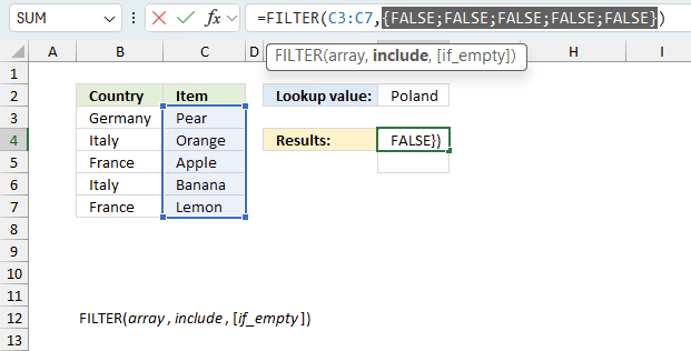
17. #CALC! error returns [if_empty] argument

The FILTER function in cell F4 returns a #CALC! error. The value in cell F2 is not found in any of the cells in B3:B7.
The FILTER function returns #CALC! error instead of an empty array. The third argument allows you to customize what to return if the FILTER function returns nothing, see below.

18. Get Excel file
Useful links
19. Lookup and return multiple sorted values based on corresponding values in another column - Excel 365
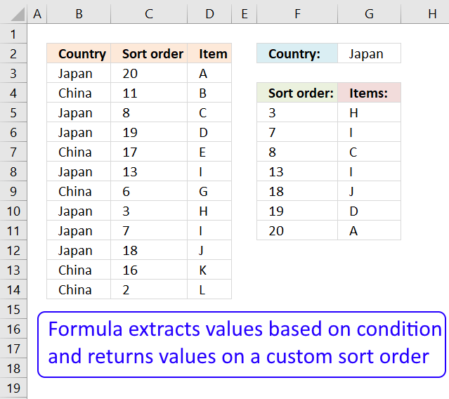
This example shows how to filter records based on a lookup value and return the result sorted based on a given column. The image above shows the data set in cells B3:D14, it has three column header names: Country, Sort order, and Item. The lookup value is in cell G2, in this example it is "Japan".
The result is displayed in cells F5:G5 and cells below as far as needed. It shows all the records from B3:D14 where B3:B14 matches the lookup value in cell G3. They match in cell s B3, B5:B6, B8, and B10:B12, the corresponding values on the same rows are shown in cells F5:G5 and cells below as far as needed sorted based on the numbers in column B named "Sort order".
Excel 365 dynamic array formula:
Explaining formula
SORTBY(FILTER(C3:D14, B3:B14=G2),INDEX(FILTER(C3:D14, B3:B14=G2),0,1))
Step 1 - Find values equal to condition
The equal sign lets you compare value to value, the result is a boolean value TRUE or FALSE.
B3:B14=G2
and returns {TRUE; FALSE; ... ; FALSE}
Step 2 - Filter values based on logical expression
The FILTER function extracts values/rows based on a condition or criteria.
Function syntax: FILTER(array, include, [if_empty])
FILTER(C3:D14, B3:B14=G2)
and returns {20,"A"; ... ,"J"}
Step 3 - Extract first column in array
The INDEX function returns a value or reference from a cell range or array, you specify which value based on a row and column number.
Function syntax: INDEX(array, [row_num], [column_num])
INDEX(FILTER(C3:D14, B3:B14=G2),0,1)
and returns {20; 8; 19; 13; 3; 7; 18}.
Step 4 - Sort array based on first column
The SORTBY function sorts a cell range or array based on values in a corresponding range or array.
Function syntax: SORTBY(array, by_array1, [sort_order1], [by_array2, sort_order2],…)
SORTBY(FILTER(C3:D14, B3:B14=G2),INDEX(FILTER(C3:D14, B3:B14=G2),0,1))
and returns {3, "H"; 7, "I"; 8, "C"; 13, "I"; 18, "J"; 19, "D"; 20, "A"}.
Step 5 - Shorten formula
The LET function lets you name intermediate calculation results which can shorten formulas considerably and improve performance.
Function syntax: LET(name1, name_value1, calculation_or_name2, [name_value2, calculation_or_name3...])
SORTBY(FILTER(C3:D14, B3:B14=G2),INDEX(FILTER(C3:D14, B3:B14=G2),0,1))
x - FILTER(C3:D14, B3:B14=G2)
LET(x,FILTER(C3:D14, B3:B14=G2),SORTBY(x,INDEX(x,0,1))
Get the Excel file
Lookup-and-return-multiple-sorted-values-based-on-corresponding-values-in-another-column-Excel-365.xlsx
20. Lookup and return multiple sorted values based on corresponding values in another column- previous Excel versions
Hi Oscar,
Thanks for creating such a helpful website and I've a question if I would like to return the value with a prefix order would it possible? If not can I just add another column in the data and used it as part of the search criteria?
The array formula in cell G5 looks for the value Japan (cell G2) in column B and returns corresponding values in column D, sorted ascending by the numbers in column C.
Formula in cell G5:
Formula in cell F5:
You can change the sort order to descending by replacing the SMALL function with the LARGE function.
How to enter an array formula
Excel 365 subscribers do not need to enter the formulas as array formulas.
- Copy above formula for cell G5 (Ctrl + c).
- Double press with left mouse button on cell G5.
- Paste array formula (CTRL + v).
- Press and hold CTRL + SHIFT simultaneously.
- Press Enter once.
- Release all keys.
The formula now has curly brackets before and after the array formula {=array_formula}, if you did the above steps correctly.
How to copy array formula to cells below
- Select cell G5.
- Copy cell (Ctrl + c).
- Select cell range G6:G11.
- Paste (Ctrl + v).
Explaining array formula in cell G5

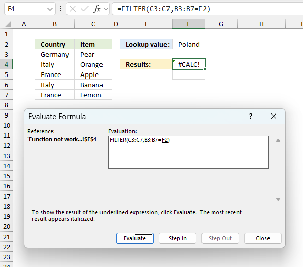
The "Evaluate Formula" tool is great for troubleshooting and examining formulas. Select the cell containing the formula you want to debug. Go to tab "Formulas", press with left mouse button on the "Evaluate Formula" button.

A dialog box appears, see image above. Press with left mouse button on the "Evaluate" button move to the next calculation step, underlined expression will be evaluated next when you press with left mouse button on the "Evaluate" button.
Text in italic is the most recent evaluated expression. Keep press with left mouse button oning the "Evaluate" button to see all steps, press with left mouse button on "Close" button to dismiss the dialog box.
Step 1 - Filter sort numbers for selected country

The IF function returns one value if the logical expression returns TRUE and another value if FALSE.
IF(logical_test, valie_if_true, value_if_false)
IF($G$2=$B$3:$B$14,$C$3:$C$14,"")
becomes
{20; ""; 8; 19; ""; 13; ""; 3; 7; 18; ""; ""}
This array is shown in column E in the image above. Only values from column C are shown based on the condition in cell G2 and the corresponding value in column B.
Step 2 - Find k-th smallest value in the array
The SMALL function returns the k-th smallest number from a cell range or an array.
SMALL(array, k)
SMALL(IF($G$2=$B$3:$B$14, $C$3:$C$14,""), ROW(A1))
becomes
SMALL({20; ""; 8; 19; ""; 13; ""; 3; 7; 18; ""; ""}, 1)
and returns 3.
ROW(A1) changes as we copy the cell to cells below, this makes the array formula dynamic meaning a new value will be returned in each cell.
Step 3 - Find the relative position of the k-th smallest value in array
The MATCH function finds the relative position of a value in a column or array.
MATCH(lookup_value, lookup_array, [match_type])
MATCH(SMALL(IF($G$2=$B$3:$B$14, $C$3:$C$14, ""),ROW(A1)), IF($G$2=$B$3:$B$14, $C$3:$C$14, ""), 0)
becomes
MATCH(3, {20; ""; 8; 19; ""; 13; ""; 3; 7; 18; ""; ""}, 0)
and returns 8. Number 3 is the eigth value in the array.
Step 4 - Return Item
The INDEX function returns a value based on row and column numbers.
INDEX($D$3:$D$14, MATCH(SMALL(IF($G$2=$B$3:$B$14, $C$3:$C$14, ""),ROW(A1)), IF($G$2=$B$3:$B$14, $C$3:$C$14, ""), 0))
and returns H in cell G5.
21. Filter and sort using an Excel Table

The image above shows an Excel Table with a filter applied to column B (Country) and sorting applied to column C (Sort order).
How to create an Excel Table

- Press with mouse on any value in the data set.
- Press CTRL + T to open the "Create Table" dialog box.
- Press OK button to apply settings and create an Excel Table.

How to filter an Excel Table based on a condition

- Press with left mouse button on the arrow button next to the column header name you want to filter.
- Disable all checkboxes except the condition you want to use. I want to filter the table based on item "Japan".
Note, press with left mouse button on the "(Select All)" checkbox to deselect all checkboxes. This saves you time if you have many checkboxes to deselect.

- Press with left mouse button on "OK" button to apply filter conditions.

21.1 How to sort a filtered Excel Table

- Press with mouse on the arrow next to the column header name you want to sort by.
- Press with mouse on "Sort Smallest to Largest" or "Sort Largest to Smallest".
- Press with left mouse button on OK button to apply sorting.
22. Function not working
The FILTER function returns
- #CALC! error if the include argument evaluates to FALSE only meaning no values match the condition.
- #NAME? error if you misspell the function name.
- propagates errors, meaning that if the input contains an error (e.g., #VALUE!, #REF!), the function will return the same error.
22.1 Troubleshooting the error value
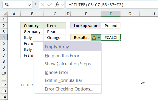
When you encounter an error value in a cell a warning symbol appears, displayed in the image above. Press with mouse on it to see a pop-up menu that lets you get more information about the error.
- The first line describes the error if you press with left mouse button on it.
- The second line opens a pane that explains the error in greater detail.
- The third line takes you to the "Evaluate Formula" tool, a dialog box appears allowing you to examine the formula in greater detail.
- This line lets you ignore the error value meaning the warning icon disappears, however, the error is still in the cell.
- The fifth line lets you edit the formula in the Formula bar.
- The sixth line opens the Excel settings so you can adjust the Error Checking Options.
Here are a few of the most common Excel errors you may encounter.
#NULL error - This error occurs most often if you by mistake use a space character in a formula where it shouldn't be. Excel interprets a space character as an intersection operator. If the ranges don't intersect an #NULL error is returned. The #NULL! error occurs when a formula attempts to calculate the intersection of two ranges that do not actually intersect. This can happen when the wrong range operator is used in the formula, or when the intersection operator (represented by a space character) is used between two ranges that do not overlap. To fix this error double check that the ranges referenced in the formula that use the intersection operator actually have cells in common.
#SPILL error - The #SPILL! error occurs only in version Excel 365 and is caused by a dynamic array being to large, meaning there are cells below and/or to the right that are not empty. This prevents the dynamic array formula expanding into new empty cells.
#DIV/0 error - This error happens if you try to divide a number by 0 (zero) or a value that equates to zero which is not possible mathematically.
#VALUE error - The #VALUE error occurs when a formula has a value that is of the wrong data type. Such as text where a number is expected or when dates are evaluated as text.
#REF error - The #REF error happens when a cell reference is invalid. This can happen if a cell is deleted that is referenced by a formula.
#NAME error - The #NAME error happens if you misspelled a function or a named range.
#NUM error - The #NUM error shows up when you try to use invalid numeric values in formulas, like square root of a negative number.
#N/A error - The #N/A error happens when a value is not available for a formula or found in a given cell range, for example in the VLOOKUP or MATCH functions.
#GETTING_DATA error - The #GETTING_DATA error shows while external sources are loading, this can indicate a delay in fetching the data or that the external source is unavailable right now.
22.2 The formula returns an unexpected value
To understand why a formula returns an unexpected value we need to examine the calculations steps in detail. Luckily, Excel has a tool that is really handy in these situations. Here is how to troubleshoot a formula:
- Select the cell containing the formula you want to examine in detail.
- Go to tab “Formulas” on the ribbon.
- Press with left mouse button on "Evaluate Formula" button. A dialog box appears.
The formula appears in a white field inside the dialog box. Underlined expressions are calculations being processed in the next step. The italicized expression is the most recent result. The buttons at the bottom of the dialog box allows you to evaluate the formula in smaller calculations which you control. - Press with left mouse button on the "Evaluate" button located at the bottom of the dialog box to process the underlined expression.
- Repeat pressing the "Evaluate" button until you have seen all calculations step by step. This allows you to examine the formula in greater detail and hopefully find the culprit.
- Press "Close" button to dismiss the dialog box.
There is also another way to debug formulas using the function key F9. F9 is especially useful if you have a feeling that a specific part of the formula is the issue, this makes it faster than the "Evaluate Formula" tool since you don't need to go through all calculations to find the issue.
- Enter Edit mode: Double-press with left mouse button on the cell or press F2 to enter Edit mode for the formula.
- Select part of the formula: Highlight the specific part of the formula you want to evaluate. You can select and evaluate any part of the formula that could work as a standalone formula.
- Press F9: This will calculate and display the result of just that selected portion.
- Evaluate step-by-step: You can select and evaluate different parts of the formula to see intermediate results.
- Check for errors: This allows you to pinpoint which part of a complex formula may be causing an error.
The image above shows cell reference B3:B7=F2 converted to hard-coded values using the F9 key. The FILTER function requires a valid array which is not the case in this example. We have found what is wrong with the formula.
Tips!
- View actual values: Selecting a cell reference and pressing F9 will show the actual values in those cells.
- Exit safely: Press Esc to exit Edit mode without changing the formula. Don't press Enter, as that would replace the formula part with the calculated value.
- Full recalculation: Pressing F9 outside of Edit mode will recalculate all formulas in the workbook.
Remember to be careful not to accidentally overwrite parts of your formula when using F9. Always exit with Esc rather than Enter to preserve the original formula. However, if you make a mistake overwriting the formula it is not the end of the world. You can “undo” the action by pressing keyboard shortcut keys CTRL + z or pressing the “Undo” button
22.3 Other errors
Floating-point arithmetic may give inaccurate results in Excel - Article
Floating-point errors are usually very small, often beyond the 15th decimal place, and in most cases don't affect calculations significantly.
'FILTER' function examples

First, let me explain the difference between unique values and unique distinct values, it is important you know the difference […]

This post explains how to lookup a value and return multiple values. No array formula required.
In this blog post I will demonstrate methods on how to find, select, and deleting blank cells and errors. Why […]
Functions in 'Lookup and reference' category
The FILTER function function is one of 25 functions in the 'Lookup and reference' category.
Excel function categories
Excel categories
19 Responses to “How to use the FILTER function”
Leave a Reply
How to comment
How to add a formula to your comment
<code>Insert your formula here.</code>
Convert less than and larger than signs
Use html character entities instead of less than and larger than signs.
< becomes < and > becomes >
How to add VBA code to your comment
[vb 1="vbnet" language=","]
Put your VBA code here.
[/vb]
How to add a picture to your comment:
Upload picture to postimage.org or imgur
Paste image link to your comment.
Hi Oscar,
This is a brilliant solution and it has help me save couple of my hairs (else will be scratching of my head on how this can be done).
Your commitment has really help us grow in out Excel knowledge and I sincerely would like to thank you for doing this.
Best Regards,
Pat
Pat,
thank you!
No array formulas
F5:
=INDEX(MOD(SMALL(($B$3:$B$14=$G$2)*($C$3:$C$14)+($B$3:$B$14<>$G$2)*10^10,ROW(A1)),10^10),0)
G5:
=IFERROR(INDEX($D$3:$D$14,MATCH(F5,INDEX(($B$3:$B$14=$G$2)*($C$3:$C$14)+($B$3:$B$14<>$G$2)*10^10,0),0),0),0)
I hope it useful
Hung,
Your formulas work, thank you for your contribution!
Mr. Oscar
Your works are all wonderful
mahmoud-lee
Thank you!
hi Oscar,
can it be sort for alphabet
momoe,
yes it can.
Array formula in cell F5:
=INDEX($D$3:$D$14, MATCH(SMALL(IF($G$2=$B$3:$B$14, COUNTIF($D$3:$D$14, "<"&$D$3:$D$14), ""), ROW(A1)), IF($G$2=$B$3:$B$14, COUNTIF($D$3:$D$14, "<"&$D$3:$D$14), ""), 0))
Array formula in cell G5:
=SMALL(IF(($G$2=$B$3:$B$14)*(F5=$D$3:$D$14), $C$3:$C$14, ""),COUNTIF($F$5:F5, F5))
Get the Excel *.xlsx file
Lookup-and-return-multiple-values-sorted-in-a-custom-order_q2.xlsx
hi Oscar, thank you.
how about lookup two value and sorted the number from small to large
Hi Oscar,
Thanks for your many great solutions.
I am trying to achieve something similar to this post, but with one major difference. Instead of sorting my results small to large or vice versa, I want only to place those results that meet a specific criteria (from another cell) at the top of the list of results, and all other results can follow in any order.
Can you help?
Simon, why would you want to include results that don't match your criteria?
Hi Oscar,
Thanks for your reply. I hadn't really appreciated that there might be some confusion over this, but I can see now!
I have an array formula, which retrieves records based on two criteria - Project Name & Status. Here is a version of the formula:
{=IF(COUNTIFS(DrugList[Project Name],$B$19,DrugList[Status],$A$24)<ROWS($C$25:C25),"",INDEX(DrugList[BNF Code],SMALL(IF((DrugList[Project Name]=$B$19)+(DrugList[Status]=$A$24)=2,ROW(DrugList[BNF Code])-1),ROW(A1))))}
This can return none, one or many (twenty or more) records, which are displayed in a list format. I want to display all of these records for comparison purposes.
However, some of the records are more important, as they match a third criteria (Strength), which is not currently included in the formula. The value for this third criteria can be referenced from a specific cell ($E$19), and regularly changes dependant upon slicer selections. The results will often contain more than one match with this third criteria, as well as many results that match the two in the array formula, but not the third criteria. I would like to be able to display all of the results which match the first two criteria in the formula (which the formula currently does), AND have the results that match the third criteria appear at the top of that list of results, with all other results displayed below, in any order.
What I can't work out, is how to get those results which match the third criteria as well as the other two, to the top of the list.
I hope that makes sense. Any help would be greatly appreciated.
Simon,
I hope this will be helpful.
Array formula in cell E6:
=INDEX($A$2:$C$9, IF(COUNTIFS($A$2:$A$9, $F$2, $B$2:$B$9, $F$3)>=ROWS($A$1:$A1), SMALL(IF(($A$2:$A$9=$F$2)*($B$2:$B$9=$F$3), MATCH(ROW($A$2:$A$9), ROW($A$2:$A$9)), ""), ROW(A1)), SMALL(IF(($A$2:$A$9=$F$2)*($B$2:$B$9<>$F$3), MATCH(ROW($A$2:$A$9), ROW($A$2:$A$9)), ""), ROW(A1)-COUNTIF($F$5:$F5, $F$3))), COLUMNS($A$1:A1))
What formula is in the F6 for your last replay?
Many thanks,
Dritan,
I am not sure I understand? Replay?
The formula in cell F5:
=SMALL(IF($G$2=$B$3:$B$14, $C$3:$C$14, ""),ROW(A1))
changes automatically to
=SMALL(IF($G$2=$B$3:$B$14, $C$3:$C$14, ""),ROW(A2))
in cell F6 when you copy cell F5 and paste to cells below.
Hi Oscar,
Thanks for your many great solutions. I am attempting to return multiple values sorted in a custom order (as you showed us in this post), but with 2 lookup criteria instead of 1. Is this possible?
Awesome formula! I really enjoyed working through it. However, I have run into a snag. I've been using this formula for sales and return information in a retail setting. Something like indexing the item based upon number of pieces or sold or returned from largest to smallest. However, when two different items have the same quantity, the formula looks up and returns the first on the list.
Ex. Formula returns
Item. Qty Item. Qty
bags 1 dress 2
shoes 2 dress 2
dress 2 bags 1
In this example, the second row should say "shoes" not dress. Is there a work around to ensure an item is repeated twice in the result?
Appreciate it!
How to combine trick 6 with trick 11, i.e.
https://i.postimg.cc/W1zRH7MM/Filter-function-criteria-edit.png
Piotr,
Great question!
Here is how to filter values that contain any of the given strings:
Formula in cell E6:
=FILTER(B3:C7, MMULT(ISNUMBER(SEARCH(TRANSPOSE(F2:F3), B3:B7))*1, ROW(F2:F3)^0))