How to use the SORT function

The SORT function lets you sort values from a cell range or array. It returns an array with a size that matches the number of values in the array argument.
The SORT function is in the Lookup and reference category and is only available to Excel 365 subscribers.
What's on this page
- Syntax
- Arguments
- Example
- What is a spilled array formula?
- What is a #SPILL! error?
- Sort a multicolumn cell range
- Sort a multicolumn cell range - multiple sort_index and sort_order
- Sort letters and numbers?
- Sort based on values in an adjacent column
- Case sensitive?
- Based on an Excel Table
- By column (vertically)?
- By column header?
- Sum numbers based on items and return totals sorted from large to small
- Based on item count
- Multicolumn cell range
- Get Excel file
- By adjacent number in every other value - Array formula
- By adjacent number in every other value - Excel 365 formula
- By adjacent number in every other value horizontally
- Get Excel file
- Based on a delimiting character (Formula)
- Based on a delimiting character (Macro)
- Function not working
- Get the Excel File here
1. Syntax
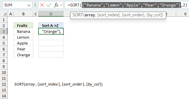
SORT(array, [sort_index], [sort_order], [by_col])
2. Arguments
| Argument | Text |
| array | Required. Cell range or array. |
| [sort_index] | Optional. A number representing the row / column to sort by. |
| [sort_order] | Optional. 1 - Ascending order (A to Z or small to large) -1 - descending order (Z to A or large to small). 1 is the default value if the argument is not specified. |
| [by_col] | Optional. False - Sort horizontally (by row), True - Sort vertically (by column). False is the default value if the argument is not specified. |
3. Example
Formula in cell D3:
The formula above sorts the data in cell range C3:C7 and returns the sorted array in cell D3.
4. What is a spilled array formula?

A spilled array formula is a formula that returns multiple values. It returns automatically all values to cells below or to the right, this is a new feature for Excel 365 subscribers.
There is no need to enter the formula as an array formula as before, simply press Enter like a regular formula.
The animated image above shows the SORT function being entered in cell D3, as soon as I press Enter the formula returns an array of values to cells below as far as needed.
5. What is a #SPILL! error?

A #SPILL! error is returned if one or more cells below are populated. The animated image above shows text value "a" in cell D6.
The SORT function in cell D3 needs cells below to show all values. Cell D6 makes this impossible and a #SPILL! error is returned in cell D3.
You have two options, delete the value in cell D6 or enter the SORT function in another cell that has empty cells below.
6. Specific column in a data set?

The SORT function can sort a multi-column cell range, however, you can only choose one column to sort by. Use the SORTBY function if you need to sort by two or more columns.
Formula in cell E3:
SORT(array, [sort_index], [sort_order], [by_col])
array - B3:C7
[sort_index] - 2
The formula in cell E3 sorts values in cell range B3:C7 based on the second column (column C) from small to large.
7. Sort a multi-column cell range - multiple sort_index and sort_order
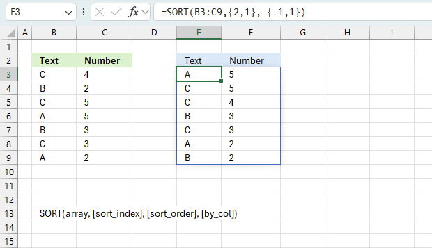
Cells B3:B9 contains letters from A to C in random order. Cell range C3:C9 contains numbers between 2 and 5 in random order.
Formula in cell E3:
=SORT(B3:C9,{2,1}, {-1,1})
The formula in cell E3 sorts the data table by the second column from large to small and then by the first column from A to Z. The SORT function allows you to specify multiple index columns by entering their relative positions inside curly brackets.
{2,1} means that the second column is to be sorted first and then the first column.
7. Is it possible to sort letters and numbers?

Yes, the SORT function sorts the numbers first and then letters if you sort from A to Z.
Formula in cell D3:
8. Sort based on an adjacent column

The image above demonstrates a formula that sorts values based on cell range B3:C7 by column 1 (B3:B7), however, it returns only column 2 (C3:C7).
Formula in cell E3:
Here is how the formula works.
Step 1 - Sort values from A to z
The SORT function sorts a cell range by the first column from A to Z with the default settings.
SORT(B3:C7)
becomes
SORT({"Banana", 5; "Lemon", 2; "Apple", 6; "Pear", 3; "Orange", 1})
and returns
{"Apple", 6; "Banana", 5; "Lemon", 2; "Orange", 1; "Pear", 3}
Step 2 - Extract the second column
The FILTER function can extract the second column using an array containing 0 (zero) and 1. The array must be the same size as the tnumber of columns in the cell range.
1 means that the column is extracted and 0 (zero) means that the column is not extracted.
FILTER(SORT(B3:C7), {0,1})
becomes
FILTER({"Apple", 6; "Banana", 5; "Lemon", 2; "Orange", 1; "Pear", 3}, {0,1})
and returns
{6; 5; 2; 1; 3}
9. Is the SORT function case sensitive?

No, it is not sorting data based on upper and lower letters. The image above shows that item "apple" and "Apple" with a capital letter is sorted in random order.
10. Sort data based on an Excel Table?

Yes, you can. Structured references work fine. Add, delete or edit values in the Excel Table and the SORT function output is instantly changed.
11. How to sort by column

The SORT function sorts an array by row if the argument is left out, however, if you use TRUE the SORT function sorts the array by column.
This is demonstrated in the image above.
Formula in cell E3:
Here is the SORT function syntax:
SORT(array, [sort_index], [sort_order], [by_col])
The last argument [by_col] lets you change the SORT method to by column. TRUE - By column, FALSE or omitted - By row.
12. How to sort by column header?

You can use the fourth argument [by_col] to sort a cell range by column header. The image above shows the formula in cell F2, the output is sorted based on column header names.
SORT(array, [sort_index], [sort_order], [by_col])
Formula in cell F2:
You can also sort the column headers from Z to A using this formula:

13. Sum numbers based on items and return totals sorted from large to small

The formula in cell F3 adds adjacent numbers based on distinct values and returns totals sorted from large to small. For example, item "Banana" is shown both in cell B3 and B7. The corresponding values are 5 and 2, the total is 7.
This calculation is made for all values in cell range B3:C7, the formula returns the totals for each item sorted from large to small in cell range F3:F5.
Formula in cell F3:
Here is how the formula works.
Step 1 - Extract unique distinct values from cell range B3:B7
The UNIQUE function returns all distinct values meaning all duplicates are merged into one distinct value.
UNIQUE(B3:B7)
becomes
UNIQUE({"Banana"; "Lemon"; "Apple"; "Lemon"; "Banana"})
and returns
{"Banana"; "Lemon"; "Apple"}
Step 2 - Add numbers based on distinct values and return totals
The SUMIF function sums values based on a condition. In this example all distinct values from cell range B3:B7 will be used as criteria.
SUMIF(range, criteria, [sum_range])
SUMIF(B3:B7, UNIQUE(B3:B7), C3:C7)
becomes
SUMIF(B3:B7, {"Banana"; "Lemon"; "Apple"}, C3:C7)
becomes
SUMIF({"Banana"; "Lemon"; "Apple"; "Lemon"; "Banana"}, {"Banana"; "Lemon"; "Apple"}, {5; 2; 8; 4; 2})
and returns
{7; 6; 8}
Step 3 - Sort numbers from large to small
SORT(SUMIF(B3:B7, UNIQUE(B3:B7), C3:C7), , -1)
becomes
SORT({7; 6; 8}, , -1)
and returns
{8; 7; 6}
Formula in cell E3
The formula in cell E3 returns the distinct values sorted based on their total shown in column F.
Step 1 - Extract distinct values
The UNIQUE function returns all distinct values meaning all duplicates are merged into one distinct value.
UNIQUE(B3:B7)
becomes
UNIQUE({"Banana"; "Lemon"; "Apple"; "Lemon"; "Banana"})
and returns
{"Banana"; "Lemon"; "Apple"}.
Step 2 - Calculate totals based on distinct values
The SUMIF function sums values based on a condition. In this example, all distinct values from cell range B3:B7 will be used as criteria.
SUMIF(range, criteria, [sum_range])
SUMIF(B3:B7, UNIQUE(B3:B7), C3:C7)
becomes
SUMIF(B3:B7, {"Banana"; "Lemon"; "Apple"}, C3:C7)
becomes
SUMIF({"Banana"; "Lemon"; "Apple"; "Lemon"; "Banana"}, {"Banana"; "Lemon"; "Apple"}, {5; 2; 8; 4; 2})
and returns
{7; 6; 8}.
Step 3 - Sort distinct values based on totals
The SORTBY function sorts an array or cell range, it has the following syntax:
SORTBY(array, by_array1, [sort_order1], [by_array2, sort_order2],…)
SORTBY(UNIQUE(B3:B7), SUMIF(B3:B7, UNIQUE(B3:B7), C3:C7), -1)
becomes
SORTBY(UNIQUE(B3:B7), {7; 6; 8}, -1)
becomes
SORTBY({"Banana"; "Lemon"; "Apple"}, {7; 6; 8},-1)
and returns
{"Apple"; "Banana"; "Lemon"}.
This article demonstrates a formula for earlier Excel versions: Extract unique distinct values sorted based on sum of adjacent values
I recommend a pivot table if you are working with lots of data: Discover Pivot Tables – Excels most powerful feature and also least known
14. Sort based on item count

The formula in cell E3 calculates the count for each distinct value and sorts the result from large to small. Item "Banan" is shown in cell B4, B6, and B8, the total count is 3 in cell range B3:B8.
The formula in cell D3 returns each distinct value from cell range B3:B8 based on their count from large to small.
Formula in cell E3:
Here is how the formula works.
Step 1 - Extract distinct values
The UNIQUE function returns all distinct values meaning all duplicates are ignored, only one instance of each value is extracted.
UNIQUE(B3:B8)
becomes
UNIQUE({"Lemon"; "Banana"; "Apple"; "Banana"; "Lemon"; "Banana"})
and returns
{"Lemon"; "Banana"; "Apple"}.
Step 2 - Count distinct values in cell range B3:B8
The COUNTIF function counts the number of cells that is equal to a condition or criteria.
COUNTIF(range, criteria)
COUNTIF(B3:B8, UNIQUE(B3:B8))
becomes
COUNTIF({"Lemon"; "Banana"; "Apple"; "Banana"; "Lemon"; "Banana"}, {"Lemon"; "Banana"; "Apple"})
and returns
{2; 3; 1}.
Step 3 - Sort the result from large to small
The SORT function sorts the array of numbers from large to small.
SORT(array, [sort_index], [sort_order], [by_col])
The second argument [sort_index] allows you to sort the array from large to small if you set it to -1.
SORT(COUNTIF(B3:B8, UNIQUE(B3:B8)), , -1)
becomes
SORT({2; 3; 1}, , -1)
and returns
{3; 2; 1}.
Formula in cell D3
Step 1 - Extract distinct values
The UNIQUE function returns all distinct values meaning all duplicates are ignored.
UNIQUE(B3:B8)
becomes
UNIQUE({"Lemon"; "Banana"; "Apple"; "Banana"; "Lemon"; "Banana"})
and returns
{"Lemon"; "Banana"; "Apple"}.
Step 2 - Count distinct values in cell range B3:B8
The COUNTIF function counts the number of cells that is equal to a condition or criteria.
COUNTIF(range, criteria)
COUNTIF(B3:B8, UNIQUE(B3:B8))
becomes
COUNTIF({"Lemon"; "Banana"; "Apple"; "Banana"; "Lemon"; "Banana"}, {"Lemon"; "Banana"; "Apple"})
and returns
{2; 3; 1}.
Step 3 - Sort the result from large to small
The SORTBY function sorts an array or cell range, it has the following syntax:
SORTBY(array, by_array1, [sort_order1], [by_array2, sort_order2],…)
SORTBY(UNIQUE(B3:B7),COUNTIF(B3:B8,UNIQUE(B3:B8)),-1)
becomes
SORTBY(UNIQUE(B3:B7),{2; 3; 1},-1)
becomes
SORTBY({"Lemon"; "Banana"; "Apple"},{2; 3; 1},-1)
and returns
{"Banana"; "Lemon"; "Apple"}.
The following article demonstrates a formula for earlier Excel versions: Sort column based on count
15. Sort a multi-column range

This example demonstrates a formula that creates an array of values from a cell range and then sorts the values.
For example, cell range B2:E5 contains numerical values and the SORT function can't sort a multicolumn cell range out of the box.
We need to convert the values to a single column array, to do that we can use the FILTERXML function. The SORT function can now easily sort the values.
Formula in cell G3:
Explaining formula in cell G3
Step 1 - Join cell values
TEXTJOIN("|",TRUE,B2:F6)
becomes
TEXTJOIN("|", TRUE, {85, 9, 28, 45, 0;40, 87, 70, 16, 0;98, 16, 97, 45, 0;70, 40, 45, 83, 0;0, 0, 0, 0, 0})
and returns
"85|9|28|45|40|87|70|16|98|16|97|45|70|40|45|83"
Step 2 - Substitute delimiting character with XML tag
SUBSTITUTE(TEXTJOIN("|",TRUE,B2:F6),"|","</B><B>")
becomes
SUBSTITUTE("85|9|28|45|40|87|70|16|98|16|97|45|70|40|45|83","|","</B><B>")
and returns
"85</B><B>9</B><B>28</B><B>45</B><B>40</B><B>87</B><B>70</B><B>16</B><B>98</B><B>16</B><B>97</B><B>45</B><B>70</B><B>40</B><B>45</B><B>83"
Step 3 - Create an array based on XML tags
FILTERXML("<A><B>"&SUBSTITUTE(TEXTJOIN("|",TRUE,B2:F6),"|","</B><B>")&"</B></A>","//B")
becomes
FILTERXML("<A><B>"&"85</B><B>9</B><B>28</B><B>45</B><B>40</B><B>87</B><B>70</B><B>16</B><B>98</B><B>16</B><B>97</B><B>45</B><B>70</B><B>40</B><B>45</B><B>83"&"</B></A>","//B")
becomes
FILTERXML("<A><B>85</B><B>9</B><B>28</B><B>45</B><B>40</B><B>87</B><B>70</B><B>16</B><B>98</B><B>16</B><B>97</B><B>45</B><B>70</B><B>40</B><B>45</B><B>83</B></A>","//B")
and returns {85; 9; 28; 45; 40; 87; 70; 16; 98; 16; 97; 45; 70; 40; 45; 83}.
Step 4 - Sort the array
SORT(FILTERXML("<A><B>"&SUBSTITUTE(TEXTJOIN("|",TRUE,B2:F6),"|","</B><B>")&"</B></A>","//B"))
becomes
SORT({85; 9; 28; 45; 40; 87; 70; 16; 98; 16; 97; 45; 70; 40; 45; 83})
and returns {9; 16; 16; 28; 40; 40; 45; 45; 45; 70; 70; 83; 85; 87; 97; 98}.
16. Get Excel file
Useful links
17. Sort items by adjacent number in every other value - Array formula
I showed you in an earlier post how to sort text by number using a formula, it was a question from Denisa. The first thing that comes to mind would be to rearrange the values and then apply a filter or an excel defined table to be able to sort the names by value.
In other words, names in one column and numbers in another column. But I didn't, I built a formula, shown in row 3 (A3:F3), it was an interesting challenge that I could not resist.
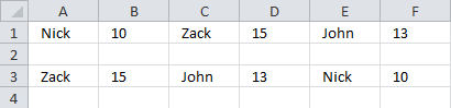
15 is the largest number and Zack is the corresponding name. 13 is the second largest number and John is the name next to it. 10 is the smallest number and the adjacent name is Nick. Check out the post if you want to know more.
In this post, I will show you a formula that sorts numbers by text, a little bit different than the previous post mentioned above. The values are in column A and the formula will sort the names alphabetically and also return the corresponding number in column C, see picture below.
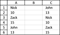
The formula is in column C.
You must enter this formula as an array formula. Here are the steps:
- Copy and paste the formula in cell C1
- Press and hold CTRL + SHIFT simultaneously
- Press Enter once
- Release all keys.
The formula is now surrounded by curly brackets, like this {=formula} if you did it right. Check your formula bar and make sure you have the curly brackets.
Then copy cell C1 and paste to cells beneath.
17.1 Explaining the formula in cell C1
Step 1 - Sort data alphabetically
The COUNTIF function counts the number of cells in a cell range that meets a condition. You can use the COUNTIF function to create an array containing numbers that represent the sort order.
COUNTIF($A$1:$A$6, "<"&$A$1:$A$6)
becomes
COUNTIF({"Nick"; 10; "Zack"; 15; "John"; 13}, "<"&{"Nick"; 10; "Zack"; 15; "John"; 13})
and returns {1; 0; 2; 2; 0; 1}
The COUNTIF function compares each value in the second argument with values in the first argument and labels them with numbers depending on their position in a sorted list. The magic is done by this code "<"& in the second argument. It appends a less than sign to each value in the second argument.
Step 2 - Filter text values
The ISTEXT function returns TRUE if a cell contains a text value and FALSE if not.
ISTEXT($A$1:$A$6)
becomes
ISTEXT({"Nick"; 10; "Zack"; 15; "John"; 13})
and returns
{TRUE; FALSE; TRUE; FALSE; TRUE; FALSE}
TRUE and FALSE are boolean values. The numerical equivalents are TRUE - 1, FALSE - 0 (zero).
Step 3 - Filter text values
The IF function returns one value if the logical test is TRUE and another value if the logical test is FALSE.
IF(logical_test, [value_if_true], [value_if_false])
IF(ISTEXT($A$1:$A$6), COUNTIF($A$1:$A$6, "<"&$A$1:$A$6), "")
becomes
IF({TRUE; FALSE; TRUE; FALSE; TRUE; FALSE}, {1; 0; 2; 2; 0; 1}, "")
and returns {1; ""; 2; ""; 0; ""}
We want to sort text values only, that is why we use the IF and ISTEXT functions to check if a value is a text value.
The double quotations "" indicate that a cell is empty.
Step 4 - Find n-th the smallest number in array
The SMALL function returns the k-th smallest value from a group of numbers.
SMALL(array, k)
SMALL(IF(ISTEXT($A$1:$A$6), COUNTIF($A$1:$A$6, "<"&$A$1:$A$6), ""), ROUND(ROW(A1)*0.5, 0))
becomes
SMALL({1;"";2;"";0;""}, ROUND(ROW(A1)*0.5, 0))
becomes
SMALL({1;"";2;"";0;""}, ROUND(0.5, 0))
becomes
SMALL({1;"";2;"";0;""}, 1)
and returns 0.
This part of the formula ROUND(ROW(A1)*0.5, 0) requires explanation, it returns a value depending on the relative cell reference A1. It changes as you copy the formula downwards. In cell C1 ROUND(ROW(A1)*0.5, 0) returns 1, C2 returns 1, C3 returns 2, C4 returns 2, C5 returns 3 and C6 returns 3. This makes it possible to get both the number and text from column A using the INDEX function, I will explain that later.
Read more about SMALL function.
Step 6 - Find the position in the array
MATCH(SMALL(IF(ISTEXT($A$1:$A$6), COUNTIF($A$1:$A$6, "<"&$A$1:$A$6), ""), ROUND(ROW(A1)*0.5, 0)), IF(ISTEXT($A$1:$A$6), COUNTIF($A$1:$A$6, "<"&$A$1:$A$6), ""), 0)
becomes
MATCH(0, IF(ISTEXT($A$1:$A$6), COUNTIF($A$1:$A$6, "<"&$A$1:$A$6), ""), 0)
becomes
MATCH(0, {1;"";2;"";0;""}, 0)
and returns 5.
Learn more about the MATCH function.
Step 7 - Return values from column A
INDEX($A$1:$A$6, MATCH(SMALL(IF(ISTEXT($A$1:$A$6), COUNTIF($A$1:$A$6, "<"&$A$1:$A$6), ""), ROUND(ROW(A1)*0.5, 0)), IF(ISTEXT($A$1:$A$6), COUNTIF($A$1:$A$6, "<"&$A$1:$A$6), ""), 0)+MOD(ROW(A2), 2))
becomes
INDEX($A$1:$A$6, 5+MOD(ROW(A2), 2))
becomes
INDEX($A$1:$A$6, 5+0)
and returns "John" from cell A5.
As you copy the formula and paste it to cells below, this part changes MOD(ROW(A2), 2). There is a relative cell reference here also, MOD(ROW(A2), 2) returns 0 in cell C1, 1 in cell C2. This makes it possible to also fetch the corresponding value.
18. Sort items by adjacent number in every other value - Excel 365 formula

Formula in cell D2:
19. Sort items by adjacent number in every other value horizontally
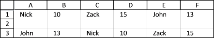
If data is arranged horisontally, see picture above. Use this array formula in cell A3:
20. Get Excel file
Back to top
21. Sort values in a single cell based on a delimiting character (Formula)

The image above shows a formula in cell D3 that sorts multiple values in cell B3 based on a delimiting character. The formula returns an array of values, Excel 365 users may enter the formula as a regular formula, however, previous versions must enter the formula as an array formula.
The FILTERXML function is an Excel 2013 function.
Formula in cell D3:
Update! The new TEXTSPLIT function available for Excel 365 users.
Excel 365 dynamic array formula in cell D3:
21.1 Explaining formula in cell D3
Step 1 - Replace the delimiting character with a XML tag name
The SUBSTITUTE function substitutes a given string with another string, all found instances are replaced.
SUBSTITUTE(B3, ",", "</a><a>")
returns "c</a><a>b</a><a>m</a><a> v</a><a> b </a><a> a"
Step 2 - Concatenate XML tags
The ampersand character concatenates strings in an excel formula.
"<b><a>"&SUBSTITUTE(B3, ",", "</a><a>")&"</a></b>"
returns "<b><a>c</a><a>b</a><a>m</a><a> v</a><a> b </a><a> a</a></b>"
Step 3 - Extract XML data
FILTERXML("<b><a>"&SUBSTITUTE(B3, ",", "</a><a>")&"</a></b>","//a")
returns {"c";"b";"m";"v";"b";"a"}.
Note that leading and trailing blanks are automatically removed.
Step 4 - Sort array values
SORT(FILTERXML("<b><a>"&SUBSTITUTE(B3, ",", "</a><a>")&"</a></b>","//a"))
returns {"a";"b";"b";"c";"m";"v"}.
22. Sort values in a single cell based on a delimiting character (Macro)
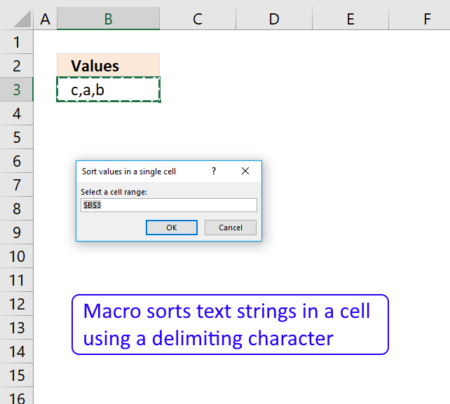
The macro asks you for a delimiting character and based on that character it creates an array of values and returns those values concatenated and sorted.
What you will learn in this section
- How to use an inputbox programmatically.
- How to iterate through cells using VBA.
- How to split values in a cell programmatically.
- How to send an array to another macro/User defined function using VBA.
- How to sort arrays from A to Z.
- How to concatenate values in an array using VBA.
22.1 How this macro works

The animated image above shows you how to start the macro and use the macro.
- Make sure you have made a backup of your workbook before running this macro.
- Press Alt + F8 to open the macro dialog box.
- Press with mouse on macro SortValuesInCell to select it.
- Press with left mouse button on "Run" button to run the macro.
- The macro shows a input box and prompts for a cell range, select a cell range.
- Press with left mouse button on OK button.
- The macro asks for a delimiting character, type it and then press OK button.
- The macro returns the values sorted in the same cells as they were fetched from.
22.2 VBA Code
'Name macro
Sub SortValuesInCell()

'Dimension variables and declare data types
Dim rng As Range
Dim cell As Range
Dim del As String
Dim Arr As Variant

'Enable error handling
On Error Resume Next

'Show an inputbox and ask for a cell range
Set rng = Application.InputBox(Prompt:="Select a cell range:", _
Title:="Sort values in a single cell", _
Default:=Selection.Address, Type:=8)

'Show an inputbox and ask for a delimiting character
del = InputBox(Prompt:="Delimiting character:", _
Title:="Sort values in a single cell", _
Default:="")

'Disable error handling
On Error GoTo 0

'Iterate through each cell in cell range
For Each cell In rng

    'Split values based on the delimiting character and save those to an array variable
    Arr = Split(cell, del)

    'Sort array using a second user defined function
    SelectionSort Arr

    'Concatenate array using the same delimiting character
    cell = Join(Arr, del)

'Continue with next cell
Next cell

End Sub
22.3 Sort algorithm
The following user defined function sorts the contents in an array.
'Name user defined function and dimension arguments and declare data types
Function SelectionSort(TempArray As Variant)

    'Dimension variables and declare data types
    Dim MaxVal As Variant
    Dim MaxIndex As Integer
    Dim i As Integer, j As Integer

    ' Step through the elements in the array starting with the
    ' last element in the array.
    For i = UBound(TempArray) To 0 Step -1

        ' Set MaxVal to the element in the array and save the
        ' index of this element as MaxIndex.
        MaxVal = TempArray(i)
        MaxIndex = i

        ' Loop through the remaining elements to see if any is
        ' larger than MaxVal. If it is then set this element
        ' to be the new MaxVal.
        For j = 0 To i
            If TempArray(j) > MaxVal Then
                MaxVal = TempArray(j)
                MaxIndex = j
            End If
        Next j

        ' If the index of the largest element is not i, then
        ' exchange this element with element i.
        If MaxIndex < i Then
            TempArray(MaxIndex) = TempArray(i)
            TempArray(i) = MaxVal
        End If
    Next i

End Function
22.4 Where to put the code?

- Copy above VBA code.
- Press Alt+ F11 to open the Visual Basic Editor.
- Select your workbook in the Project Explorer.
- Press with mouse on "Insert" on the menu.
- Press with mouse on "Module" to create a module.
- Paste VBA code to code module.
- Return to Excel.
I used the "Sort array" function found here:
Using a Visual Basic Macro to Sort Arrays in Microsoft Excel (Microsoft)
Edit: That link is now broken and I don't know where the code is located now, I have added the SelectionSort function code to this article with some small modifications.
23. Function not working
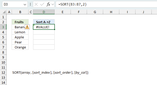
The SORT function returns
- #VALUE! error if the optional arguments are invalid.
- #NAME? error if you misspell the function name.
- propagates errors, meaning that if the input contains an error (e.g., #VALUE!, #REF!), the function will return the same error.
23.1 Troubleshooting the error value
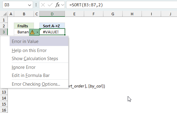
When you encounter an error value in a cell a warning symbol appears, displayed in the image above. Press with mouse on it to see a pop-up menu that lets you get more information about the error.
- The first line describes the error if you press with left mouse button on it.
- The second line opens a pane that explains the error in greater detail.
- The third line takes you to the "Evaluate Formula" tool, a dialog box appears allowing you to examine the formula in greater detail.
- This line lets you ignore the error value meaning the warning icon disappears, however, the error is still in the cell.
- The fifth line lets you edit the formula in the Formula bar.
- The sixth line opens the Excel settings so you can adjust the Error Checking Options.
Here are a few of the most common Excel errors you may encounter.
#NULL error - This error occurs most often if you by mistake use a space character in a formula where it shouldn't be. Excel interprets a space character as an intersection operator. If the ranges don't intersect an #NULL error is returned. The #NULL! error occurs when a formula attempts to calculate the intersection of two ranges that do not actually intersect. This can happen when the wrong range operator is used in the formula, or when the intersection operator (represented by a space character) is used between two ranges that do not overlap. To fix this error double check that the ranges referenced in the formula that use the intersection operator actually have cells in common.
#SPILL error - The #SPILL! error occurs only in version Excel 365 and is caused by a dynamic array being to large, meaning there are cells below and/or to the right that are not empty. This prevents the dynamic array formula expanding into new empty cells.
#DIV/0 error - This error happens if you try to divide a number by 0 (zero) or a value that equates to zero which is not possible mathematically.
#VALUE error - The #VALUE error occurs when a formula has a value that is of the wrong data type. Such as text where a number is expected or when dates are evaluated as text.
#REF error - The #REF error happens when a cell reference is invalid. This can happen if a cell is deleted that is referenced by a formula.
#NAME error - The #NAME error happens if you misspelled a function or a named range.
#NUM error - The #NUM error shows up when you try to use invalid numeric values in formulas, like square root of a negative number.
#N/A error - The #N/A error happens when a value is not available for a formula or found in a given cell range, for example in the VLOOKUP or MATCH functions.
#GETTING_DATA error - The #GETTING_DATA error shows while external sources are loading, this can indicate a delay in fetching the data or that the external source is unavailable right now.
23.2 The formula returns an unexpected value
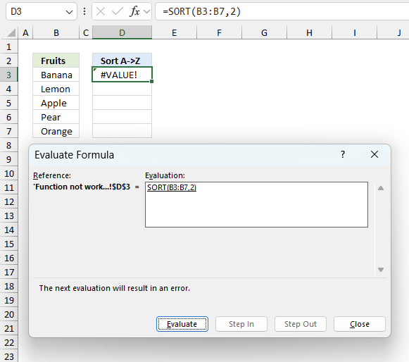
To understand why a formula returns an unexpected value we need to examine the calculations steps in detail. Luckily, Excel has a tool that is really handy in these situations. Here is how to troubleshoot a formula:
- Select the cell containing the formula you want to examine in detail.
- Go to tab “Formulas” on the ribbon.
- Press with left mouse button on "Evaluate Formula" button. A dialog box appears.
The formula appears in a white field inside the dialog box. Underlined expressions are calculations being processed in the next step. The italicized expression is the most recent result. The buttons at the bottom of the dialog box allows you to evaluate the formula in smaller calculations which you control. - Press with left mouse button on the "Evaluate" button located at the bottom of the dialog box to process the underlined expression.
- Repeat pressing the "Evaluate" button until you have seen all calculations step by step. This allows you to examine the formula in greater detail and hopefully find the culprit.
- Press "Close" button to dismiss the dialog box.
There is also another way to debug formulas using the function key F9. F9 is especially useful if you have a feeling that a specific part of the formula is the issue, this makes it faster than the "Evaluate Formula" tool since you don't need to go through all calculations to find the issue.
- Enter Edit mode: Double-press with left mouse button on the cell or press F2 to enter Edit mode for the formula.
- Select part of the formula: Highlight the specific part of the formula you want to evaluate. You can select and evaluate any part of the formula that could work as a standalone formula.
- Press F9: This will calculate and display the result of just that selected portion.
- Evaluate step-by-step: You can select and evaluate different parts of the formula to see intermediate results.
- Check for errors: This allows you to pinpoint which part of a complex formula may be causing an error.
The image above shows cell reference B3:B7 converted to hard-coded value using the F9 key.
Tips!
- View actual values: Selecting a cell reference and pressing F9 will show the actual values in those cells.
- Exit safely: Press Esc to exit Edit mode without changing the formula. Don't press Enter, as that would replace the formula part with the calculated value.
- Full recalculation: Pressing F9 outside of Edit mode will recalculate all formulas in the workbook.
Remember to be careful not to accidentally overwrite parts of your formula when using F9. Always exit with Esc rather than Enter to preserve the original formula. However, if you make a mistake overwriting the formula it is not the end of the world. You can “undo” the action by pressing keyboard shortcut keys CTRL + z or pressing the “Undo” button
23.3 Other errors
Floating-point arithmetic may give inaccurate results in Excel - Article
Floating-point errors are usually very small, often beyond the 15th decimal place, and in most cases don't affect calculations significantly.
24. Get Excel *.xlsx file
'SORT' function examples

This post explains how to lookup a value and return multiple values. No array formula required.
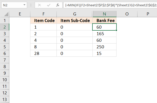
This article describes an array formula that compares values from two different columns in two worksheets twice and returns a […]
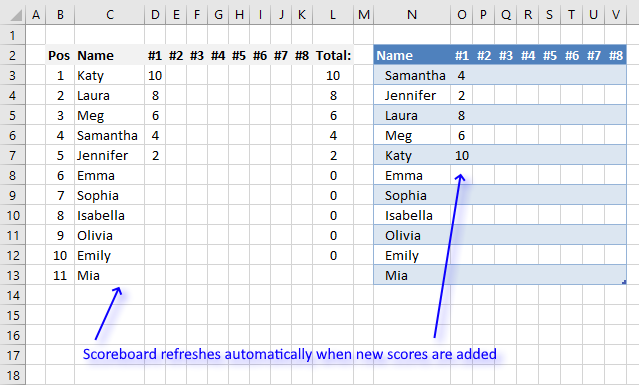
This article demonstrates a scoreboard, displayed to the left, that sorts contestants based on total scores and refreshes instantly each […]
Functions in 'Lookup and reference' category
The SORT function function is one of 25 functions in the 'Lookup and reference' category.
Excel function categories
Excel categories
8 Responses to “How to use the SORT function”
Leave a Reply
How to comment
How to add a formula to your comment
<code>Insert your formula here.</code>
Convert less than and larger than signs
Use html character entities instead of less than and larger than signs.
< becomes < and > becomes >
How to add VBA code to your comment
[vb 1="vbnet" language=","]
Put your VBA code here.
[/vb]
How to add a picture to your comment:
Upload picture to postimage.org or imgur
Paste image link to your comment.
this code doesn't sort the natural numbers
1. this way: 0, 1, 2, 3, 11, 15, 22
2. code is sorting this way : 0, 1, 11, 15, 2, 22, 3
will it be possible to sort in no.1 type...?
Thanks!
Really helpful!
[…] How to sort values in one cell using a custom delimiter [Get Digital Help] […]
[…] How to sort values in one cell using a custom delimiter [Get Digital Help] […]
I opened your cell.xlsm spreadsheet example. It worked for the most part except it placed the first entry in the cell list at the end. I assume because it was the only value not preceded by a comma.
How do I fix that? Thanks, Jeff
Hi,I’m trying to sort values in particular cell that contains 1/6/unverified/2, I need to change them to 1/6/2/unverified i.e., the work unverified should come to last in a cell. Can you help me how to do this using vba
how to transpose data in MSExcel?
e.g
Name
Age
Sex
will become
Name|Age|Sex,.....
TRANSPOSE function
TEXTJOIN function