Extract unique distinct values from a multi-column cell range

This article demonstrates ways to list unique distinct values in a cell range with multiple columns. The data is not arranged so values belong to each other row by row, this article demonstrates how to list unique distinct rows.
Table of Contents
1. Extract unique distinct values from a multi-column cell range - Excel 365
Excel 365 formula in cell B8:
Explaining formula in cell B8
Step 1 - Rearrange data to a single column array
The TOCOL function rearranges values in 2D cell ranges to a single column.
Function syntax: TOCOL(array, [ignore], [scan_by_col])
TOCOL(B2:D4)
Step 2 - List unqiue distinct values
The UNIQUE function returns a unique or unique distinct list.
Function syntax: UNIQUE(array,[by_col],[exactly_once])
UNIQUE(B2:D4)
2. Extract unique distinct values from a multi-column cell range - earlier Excel versions
Question: I have cell values spanning over several columns and I want to create a unique list from that range. How?
Answer:
Thanks to Eero, who contributed the original array formula!

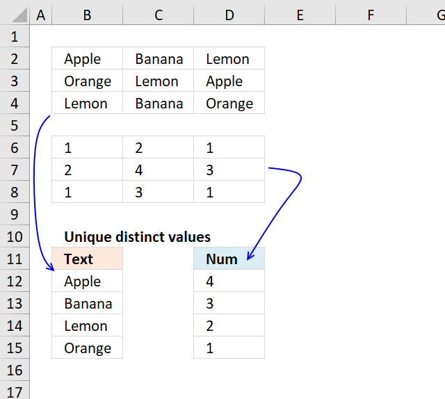
Unique distinct text values from range tbl_text, array formula in B13:
2.1 How to enter an array formula
- Double press with left mouse button on cell B13.
- Copy and paste above formula to cell B13.
- Press and hold CTRL + SHIFT simultaneously.
- Press Enter once.
- Release all keys.
Your formula now looks like this: {=array_formula}
Don't enter these characters yourself, they appear automatically when you do above steps.
2.2 How to copy array formula
Copy cell B13 and paste it down as far as necessary.
2.3 Explaining array formula in cell B13
The array formula has two parts. One part returns row numbers and the other part returns column numbers. Let us begin with the first part, returning row numbers.
Step 1 - Find new unique distinct text values
The COUNTIF function calculates the number of cells that is equal to a condition.
Function syntax: COUNTIF(range, criteria)
COUNTIF($B$12:B12, tbl_text)=0
returns {TRUE,TRUE,... ,TRUE}.
Step 2 - Convert boolean array to row numbers
The COUNTIF function calculates the number of cells that is equal to a condition.
Function syntax: COUNTIF(range, criteria)
IF(COUNTIF($B$12:B12, tbl_text)=0, ROW(tbl_text)-MIN(ROW(tbl_text))+1)
returns {1,1,1;... ,3}
Step 3 - Extract smallest value in array
The MIN function returns the smallest number in a cell range.
Function syntax: MIN(number1, [number2], ...)
MIN(IF(COUNTIF($B$12:B12, tbl_text)=0, ROW(tbl_text)-MIN(ROW(tbl_text))+1))
becomes MIN({1,1,1;2,2,2;3,3,3}) and returns 1.
Step 4 - Part two, identify array values in current row
The INDEX function returns a value or reference from a cell range or array, you specify which value based on a row and column number.
Function syntax: INDEX(array, [row_num], [column_num])
INDEX(tbl_text, MIN(IF(COUNTIF($B$12:B12, tbl_text)=0, ROW(tbl_text)-MIN(ROW(tbl_text))+1)), , 1))
returns array {"Apple", "Banana", "Lemon"}
Step 5 - Find new unique distinct text values in current row
The COUNTIF function calculates the number of cells that is equal to a condition.
Function syntax: COUNTIF(range, criteria)
COUNTIF($B$12:B12, INDEX(tbl_text, MIN(IF(COUNTIF($B$12:B12, tbl_text)=0, ROW(tbl_text)-MIN(ROW(tbl_text))+1)), , 1))
becomes COUNTIF("Text", {"Apple", "Banana", "Lemon"}) and returns {0,0,0}
Step 6 - Find a new unique distinct text value in current row
The MATCH function returns the relative position of an item in an array that matches a specified value in a specific order.
Function syntax: MATCH(lookup_value, lookup_array, [match_type])
MATCH(0, COUNTIF($B$12:B12, INDEX(tbl_text, MIN(IF(COUNTIF($B$12:B12, tbl_text)=0, ROW(tbl_text)-MIN(ROW(tbl_text))+1)), , 1)), 0)
becomes MATCH(0, {0,0,0}, 0) and returns 1.
Step 7 - Get value
The INDEX function returns a value or reference from a cell range or array, you specify which value based on a row and column number.
Function syntax: INDEX(array, [row_num], [column_num])
INDEX(tbl_text, MIN(IF(COUNTIF($B$12:B12, tbl_text)=0, ROW(tbl_text)-MIN(ROW(tbl_text))+1)), MATCH(0, COUNTIF($B$12:B12, INDEX(tbl_text, MIN(IF(COUNTIF($B$12:B12, tbl_text)=0, ROW(tbl_text)-MIN(ROW(tbl_text))+1)), , 1)), 0), 1)
becomes
INDEX(tbl_text, 1, 1)
and returns value "Apple" in cell B13.
Explaining array formula in cell D13
Step 1 - Remove previously extracted values above current cell with an array with boolean values
The COUNTIF function calculates the number of cells that is equal to a condition.
Function syntax: COUNTIF(range, criteria)
COUNTIF($D$12:D12, tbl_num)=0
becomes {0,0,... ,0}=0 and returns {TRUE,TRUE,... ,TRUE}
Step 2 - Convert boolean values to numeric values
The IF function returns one value if the logical test is TRUE and another value if the logical test is FALSE.
Function syntax: IF(logical_test, [value_if_true], [value_if_false])
IF(COUNTIF($D$12:D12, tbl_num)=0, tbl_num, "")
returns {1, 2, 1;2, 4, 3;1, 3, 1}
Step 3 - Convert boolean values to numeric values
The LARGE function calculates the k-th largest value from an array of numbers.
Function syntax: LARGE(array, k)
LARGE(IF(COUNTIF($D$12:D12, tbl_num)=0, tbl_num, ""), 1)
becomes
LARGE({1, 2, 1;2, 4, 3;1, 3, 1}, 1)
and returns 4 in cell D13.
Useful resources
UNIQUE function - Microsoft
TOCOL function - Microsoft
Unique distinct values category

First, let me explain the difference between unique values and unique distinct values, it is important you know the difference […]
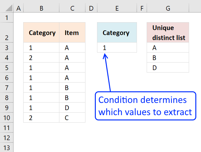
This article shows how to extract unique distinct values based on a condition applied to an adjacent column using formulas. […]
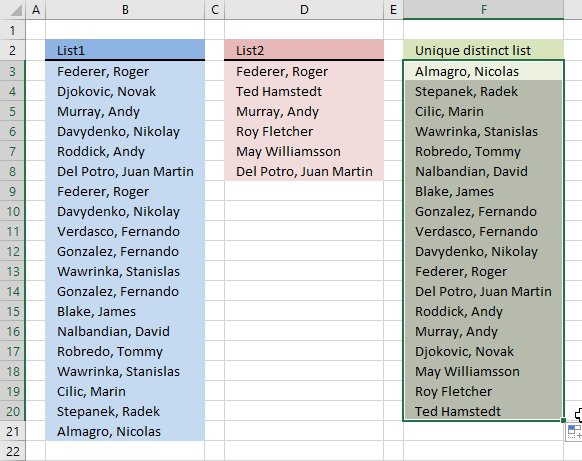
Question: I have two ranges or lists (List1 and List2) from where I would like to extract a unique distinct […]
Excel categories
25 Responses to “Extract unique distinct values from a multi-column cell range”
Leave a Reply
How to comment
How to add a formula to your comment
<code>Insert your formula here.</code>
Convert less than and larger than signs
Use html character entities instead of less than and larger than signs.
< becomes < and > becomes >
How to add VBA code to your comment
[vb 1="vbnet" language=","]
Put your VBA code here.
[/vb]
How to add a picture to your comment:
Upload picture to postimage.org or imgur
Paste image link to your comment.
A slightly different approach to extract unique items from a N*M table (named as "tbl" in the formula).
So type say "Unique items from the table" in A1 and enter the following formula as an array into A2 and copy it down as far as necessary.(it is supposed column A to be free)
=INDEX(tbl,MIN(IF(COUNTIF($A$1:A1,tbl)=0,ROW(tbl)-MIN(ROW(tbl))
+1)),MATCH(0,COUNTIF($A$1:A1,INDEX(tbl,MIN(IF(COUNTIF($A$1:A1,tbl)=0,ROW(tbl)-MIN
(ROW(tbl))+1)),,1)),0),1)
Thank you! Your formula is working perfectly! No need for a "helper" column!
Hi,
How I can extend "tbl_text" as reported in your example??
I need to enlarge that range for a bigger table.
Thanks,
Fabio,
Use "Name Manager" to change range.
https://office.microsoft.com/en-us/excel-help/define-and-use-names-in-formulas-HA010147120.aspx
It works now!
Many thanks,
Fabio
If a blank cell is located anywhere in the tbl, the formula returns the blank. I guess technically a blank is a unique value in the tbl but I'm trying to make sure only relevant numbers are returned. Any thoughts on how to correct this?
Curious,
Get the example file:
Unique-distinct-values-from-multiple-columns-using-array-formulas-without-blanks.xls
Hi Oscar,
at the end there is a #N/A in this file can you please suggest me how to get rid of it.
thanks for your help.
Sandeep,
=IFERROR(formula, "")
I have tried the formulas in this article and some from other articles and comments, but none have worked for my particular problem. I'd appreciate any help/insight.
I have several worksheets, each with a table inserted. I would like to create the list of uniques in the column of the summary worksheet's table. The methods on this site work for creating a list from a 1/2/3 columns, but fails for multiple columns (in my case). I have 4 and I'd rather understand the "general" approach than keep creating ever more convoluted formulas as columns increase.
I have created a named range that spans 4 worksheets (in the Name Manager - Name: MultiPC Refers To=A[PC],B[PC],C[PC],D[PC] -- references 4 table columns on separate worksheets).
The formulas create several errors. Stepping through them, when it tries to evaluate INDEX(*MultiPC*,... it says that it will result in an error. The value for MultiPC shown below the formula is the absolute references for MultiPC (comma separated between sheets, e.g. Sheet1!$B$2:$B$31,Sheet2!$B$2:$B:23...).
I'm guessing it's because the named range doesn't consitute an array (not rectangular? is this the case with all non-contiguous ranges?). I'm not really sure if that's the problem and how to tackle it. I've thought about making hidden columns in a single worksheet for the unique list of each worksheet, then applying this approach. Another alternative might be to extend the 3-column method from here https://www.get-digital-help.com/2009/06/20/extract-a-unique-distinct-list-from-three-columns-in-excel/ (add another nested IFERROR(INDEX...MATCH(...COUNTIF(... ), but again, I'm trying to learn a general solution that doesn't require an ever-expanding formula.
Of course, it'd be a cinch if I was allowed to use VBA for this project, but our workplace doesn't allow macros, so I'm stuck using formulas at the moment. What's your opinion? Thanks a lot!
So, I almost have it set. Using either of your array formulas below for refering to a 4-column list, I'm having trouble with a "0" (zero) being placed when blank cells are in the referenced columns. Any ideas of how to eliminate this zero? If I reference 3 columns only, there's no problem. by the way, thanks so much for the info on your website.
=IFERROR(IFERROR(IFERROR(IFERROR(INDEX(List1, MATCH(0, COUNTIF($E$1:E1, List1), 0)), INDEX(List2, MATCH(0, COUNTIF($E$1:E1, List2), 0))), INDEX(List3, MATCH(0, COUNTIF($E$1:E1, List3), 0))), INDEX(List4, MATCH(0, COUNTIF($E$1:E1, List4), 0))), "")
=IFERROR(INDEX($B$15:$D$64, MIN(IF((COUNTIF($F$14:$F14, $B$15:$D$64)=0)*($B$15:$D$64""), ROW($B$15:$D$64)-MIN(ROW($B$15:$D$64))+1)), MATCH(0, COUNTIF($F$14:$F14, INDEX($B$15:$D$64, MIN(IF((COUNTIF($F$14:$F14, $B$15:$D$64)=0)*($B$15:$D$64""), ROW($B$15:$D$64)-MIN(ROW($B$15:$D$64))+1)), , 1)), 0), 1),"")
Colin,
See this workbook:
https://www.get-digital-help.com/wp-content/uploads/2014/10/Unique-distinct-values-from-four-ranges-with-blanks.xlsx
Named ranges
List1:=Sheet1!$A$1:$A$7
List2:=Sheet1!$C$1:$C$7
List3:=Sheet1!$E$1:$E$7
List4:=Sheet1!$G$1:$G$8
Zeta,
I have several worksheets, each with a table inserted. I would like to create the list of uniques in the column of the summary worksheet's table. The methods on this site work for creating a list from a 1/2/3 columns, but fails for multiple columns (in my case). I have 4 and I'd rather understand the "general" approach than keep creating ever more convoluted formulas as columns increase.
Here is an example of four columns:
how-to-extract-a-unique-list-from-four-columns-in-excel.xlsx
I'm guessing it's because the named range doesn't consitute an array (not rectangular? is this the case with all non-contiguous ranges?). I'm not really sure if that's the problem and how to tackle it. I've thought about making hidden columns in a single worksheet for the unique list of each worksheet, then applying this approach. Another alternative might be to extend the 3-column method from here https://www.get-digital-help.com/2009/06/20/extract-a-unique-distinct-list-from-three-columns-in-excel/ (add another nested IFERROR(INDEX...MATCH(...COUNTIF(... ), but again, I'm trying to learn a general solution that doesn't require an ever-expanding formula.
I am sorry, I don´t have a general solution to this problem.
Oscar,
I really appreciate your reply. Your site is an incredible resource. I used the 4-column formula you provided, but if I find a method that works for N columns across multiple sheets, I will let the folks here know!
Thanks again,
Z
Thank you for writing this, it works like a charm!
However, there is one thing I would like to do different:
When I enter more entries in the array, the list updates with new entries in the order of first looking through the row, then going down the column. I would prefer the list first list the unique values in the column going downward, then then next column downward etc. Is that possible?
Thank you
Jonas,
See this file:
Unique-distinct-values-from-multiple-columns-using-array-formulas-jonas.xls
If the Range : tbl_num contains the numbers of :
Apple Banana Lemon
Orange Lemon Apple
Lemon Banana Orange
50 70 80
22 15 18
17 20 25
How to calculate the numbers of Apple , Banana , Lemon , Orange
Khaled Ali
Please explain in greater detail, what is the desired output?
[...] The answer is that there is no need for multiple duplicate columns in the array. Excel simplifies the array down to a single column. But when used with multiple cell ranges in more complicated array formulas, make sure the number of rows match. See this example: Unique distinct values from a cell range [...]
[…] As the name also implies, the data in G2:J14 is expected to be text with length > 0. Source. Unique distinct values from multiple columns using array formula | Get Digital Help - Microsoft Exce… The basic MATCH/COUNTIF has been attributed to Eero (a contributor at the now defunct MS […]
I realize this is an old thread but its the closest I have been able to get to a solution for my problem. I am working with a data set spread across multiple sheets. I am pulling unique distinct a-z sorted values from a column with a single criteria. I am using a helper column on my "summary" sheet for each of the sheets I pull data from. I am then combining this into a unique distinct sorted list without blanks. The "summary" page is getting quite processor intensive with all the helper columns I am using. Is there a way to add a single criteria element to the formula? Basically a Unique distinct sorted list from two columns with a single criteria removing blanks?
I am interested in counting unique values across 8 columns in Excel that are not adjoining (i.e. AF, AN, AV, BD, BL, BT, CB, CJ). I have found functions to count in one or two columns but nothing for 8 and I cannot adapt them for my issue. Any suggestions?
Very helpful article - many thanks for posting the formula and the explanation. It did exactly as specified on the tin.
Great Formula! Thank You for posting and keeping it here.
Hi,
I have more than 20 columns with true and false values. How do i get the names of top ten column with true values?