How to use the COUNTIF function

What is the COUNTIF function?

The COUNTIF function calculates the number of cells that meet a given condition.

The image above shows names in cell range B3:B10, the formula in cell D3 counts the cells in B3:B10 equal to a specified condition. The condition in this example is "Lucy".

Formula in cell D3:

Lucy is found twice, in cell B3 and B7, the function returns 2 in cell D3.

The condition is not case sensitive meaning condition "lucy" will also return 2 demonstrated in the image above.

Note that you can use multiple conditions in the second argument, however, you need to enter the formula as an array formula. Excel 365 subscribers don't need to enter the formula as an array formula.

1. Syntax

COUNTIF(range, criteria)

Back to top

2. Arguments

range	Required. The cell range you want to count the cells meeting a condition.
criteria	Required. The condition that you want to count.

Back to top

3. How to count cells equal to a condition?

The following formula in cell F6 counts the number of cells within cell range C6:C13 that equals the condition specified in cell F5.

You can also use a value instead of a cell reference inside the formula.

Name "Lucy" is hardcoded into the formula in this example. Hardcoded values mean that the formula contains literal values and cell references are not being used.

The downside is that you need to change the formula if you need to use another value.

Cell reference C6:C13 is a relative cell reference meaning it will change if you copy the cell (not the formula) and paste it to other cells. Add dollar signs, to prevent this behavior, which will lock the cell reference. Example, $C$6:$C$13.

To toggle between relative and absolute cell references you select the cell reference and then press function key F4. To learn more, read this article:
How to use absolute and relative references

COUNTIF(C6:C13, "Lucy")

Note that the array has semicolons as a separating character, which shows that the values are located on a row each.

You can easily convert a cell reference to hardcoded values, select the cell range and then press function key F9. That will instantly convert the cell range to constants.

COUNTIF({"Lucy"; "Elizabeth"; "Martin"; "Andrew"; "Lucy"; "Jennifer"; "Geoffrey"; "Abraham"}, "Lucy")

returns 2 in cell D5. I have bolded the matching values to show that the correct value is 2.

Back to top

4. Example 2 - Count cells larger/less than a criterion

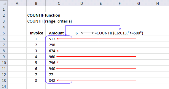
The following formula in cell D5 counts the number of cells within cell range C6:C13 that is larger than or equal to 500. The image above has six numbers in cell range C6:C14 that are larger than or equal to 500.

The formula in cell D5 returns 6, the following six numbers 512, 674, 960, 796, 940 and 848 are larger than 500.

You can use these operators:

• < less than
• > larger than
• = equal sign
• <= less than or equal to
• >=larger than or equal to
• <> not equal to

Remember to use double quotes when you combine a number with an operator.

Back to top

5. Example 3 - Count cells containing a text string

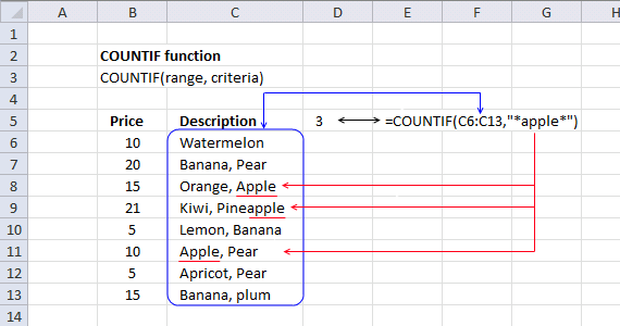
The following formula in cell D5 counts the number of cells within cell range C6:C13 that contains the text string "apple":

The asterisk matches no characters, any single character or any multiple characters. That is why "*apple*" matches "Orange, Apple", note also that the COUNTIF function is not taking into account upper and lower letters.

There is one more wildcard character you can use which is the question mark. The question mark allows you to match any single character.

The formula above utilizes this condition "*appl?" and matches two cells in cell range C6:C13, displayed in the above image. They are "Orange, Apple" and "Kiwi, Pineapple".

Back to top

6. Example 4 - running count

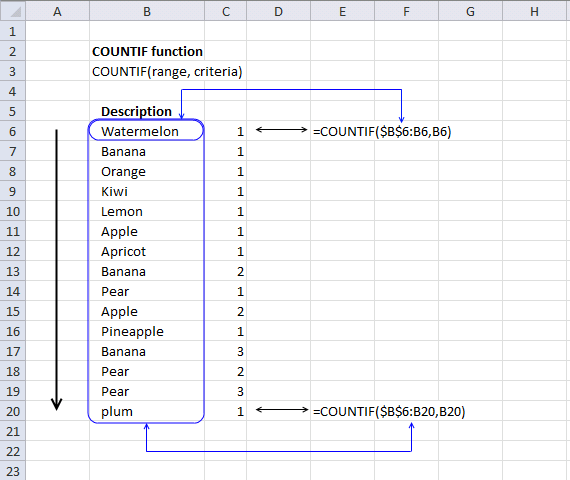
With clever use of absolute and relative cell references you can build formulas containing cell references that expand automatically when you copy the cell and paste to cells below. This example shows a "running count" meaning as the formula is copied to cells below as far as needed the calculations include new values next to the formula cell making it "running".

Formula in cell C6:

$B$6:B6 is a cell reference to cell B6. When the cell is copied to cells below, the cell reference changes. The first part $B$6 i always locked to cell B6, the last part B6 changes. Cell range $B$6:B6 "grows" when you copy the cell.

This technique is used in this popular post: Filter unique distinct values

In cell C20:

returns 1 in cell C20

Back to top

7. Example 5 - create an array of values containing the count of each value

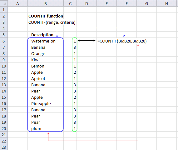
This example shows how you can use the COUNTIF function to count each value in a cell range then create an array as large as the source data range containing each count. This technique is very useful for determining unique, unique distinct , or duplicate values in a given cell range.

Array formula in cell range C6:C20:

The image above shows example data in cell range B6:B20, it contains random fruits, some are duplicates, some are unique. The array shown in cell range C6:C20 corresponds to the same item in B6:B20 meaning the number represents the count/frequency of that particular value.

For example, the first value is "Watermelon" in B6, the corresponding value in cell C6 is 1. It represents the total count of "Watermelon" in cell range B6:B20. 1 means that it is a unique value, in other words it exists only once.

The amazing thing is that Excel calculates this array in only one formula, this makes it possible to do some seriously complicated stuff with arrays.

7.1 How to enter an array formula

1.  Select cell range C6:C20
2. Copy / Paste formula to formula bar
   
3. Press and hold CTRL + SHIFT
4. Press Enter
5. Release all keys

7.2 Explaining the array formula

The COUNTIF function counts the number of cells within a range that meet a single criterion. In this example, I am using multiple values in the criteria argument.

Each value is in the criteria argument is used as a criterion and the returning array has the same number of values as the criteria argument.

The technique described here is used in this popular post: Count unique distinct values

returns {1; 3; ... ; 1} in cell range C6:C20.

Back to top

8. How to count cells containing x number of characters?

Here is one downside with the COUNTIF function, you can't use other functions in the range argument. There are rare exceptions, one is the OFFSET function.

The image above shows numbers in B6:B13 and names in C6:c13, the formula in cell F6 tries to count cells containing a value with a specific character count specified in cell F5. To do that we need to calculate the length of each value in C6:C13, however, the COUNTIF function does not allow us to preform additional calculations in the range argument.

The following formula won't work in cell F6:

=COUNTIF(LEN(C6:C13), F5)

Excel shows this dialog box containing an error message.

We need a workaround, the following formula works:

=SUMPRODUCT((LEN(C6:C13)=F5)*1)

It counts all cells in C6:C13 containing a value with 6 characters. There are two cells with 6 characters each, they are C8 and C9.

Back to top

8.1 Explaining formula in cell F6

The Evaluate Formula tool is located on the Formulas tab in the Ribbon. It is a useful feature that allows you to step through and evaluate complex formulas to understand how the calculation is being performed and identify any errors or issues. The following steps shows these detailed evaluations for the formula above.

Step 1 - Count characters for each cell

The LEN function counts the number of characters in a cell, the LEN function returns an array of numbers if you use a cell range.

LEN(C6:C13)

returns {4; 9; 6; 6; 4; 8; 8; 7}.

Step 2 - Compare with the number in cell F5

The equal sign allows you to compare values. We want to identify cells that have the same number of characters as the specified number in cell F5.

The logical expression returns TRUE or FALSE.

LEN(C6:C13)=F5

returns {FALSE; FALSE; ...; FALSE}

Step 3 - Multiply with 1

The SUMPRODUCT can't sum boolean values, we need to convert them to their numerical equivalents. TRUE = 1, FALSE = 0 (zero).

(LEN(C6:C13)=F5)*1

returns {0;0;1;1;0;0;0;0}.

Step 4 - Sum numbers

The SUMPRODUCT function is able to add numbers in an array without the need to enter the formula as an array formula.

The formula becomes slightly larger compared to using the SUM function.

SUMPRODUCT((LEN(C6:C13)=F5)*1)

Back to top

9. Dynamic array formula (Excel 365)

You no longer need to enter the formula as an array formula if you are a subscriber of Office 365, the new feature is called "Dynamic Arrays" and was introduced to Excel in January 2020.

It will automatically detect if a formula returns more than one value and will extend accordingly based on the number of values that are being returned, this is called spilling.

The image above demonstrates this behavior, the formula has extended automatically to cells below as far as needed. A blue border indicates that spilling has occurred, however, it will disappear as soon as you press with left mouse button on outside the formula range.

A #SPILL error is displayed if the destination cells are not empty. Make sure to delete cell values below and/or to the right as far as needed or enter the formula in cell that allows you to spill values below etc.

Back to top

 

11. Use IF + COUNTIF to evaluate multiple conditions

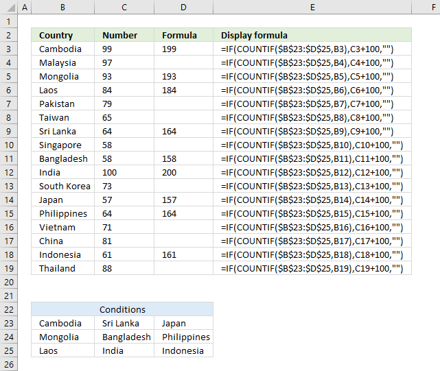
The image above demonstrates a formula that matches a value to multiple conditions, if the condition is met the formula takes the value in a corresponding cell on the same row and adds a given number.

Table of contents

1. Use IF + COUNTIF to evaluate multiple conditions
2. Use IF + COUNTIF to evaluate multiple conditions and different outcomes
3. Get Excel file
4. Filter a data set based on thousands of conditions - Excel Table, Autofilter

The COUNTIF function allows you to construct a small IF formula that carries out plenty of logical expressions.

Combining the IF and COUNTIF functions also let you have almost any number of logical expressions and the effort to type the formula is minimal.

11.1. Use IF + COUNTIF to evaluate multiple conditions

The example shown in the above picture checks if the country in cell B3 is equal to one of the countries in cell range B23:D25. If the country matches one of the conditions 100 is added to the number in cell C3.

Formula in cell D3:

In other words, the COUNTIF function counts how many times a specific value is found in a cell range. If the value exists at least once in the cell range the IF function adds 100 to the value in C3. If FALSE the formula returns a blank or empty cell.

Use the following formula if you want the same number in cell D3 if a country is not a match to any of the conditions.

=IF(COUNTIF($B$23:$D$25,B3),C3+100,C3)

For example, cell D4 checks if "Malaysia" is in any of the cells in cell range B23:D25. It is not found and the formula returns the value in cell C4.

11.1.1 Explaining formula in cell D3

Step 1 - COUNTIF function syntax

The COUNTIF function calculates the number of cells that is equal to a condition.

COUNTIF(range, criteria)

Step 2 - Populate COUNTIF function arguments

COUNTIF(range, criteria)

becomes

COUNTIF($B$23:$D$25,B3)

range - A reference to all conditions: $B$23:$D$25

criteria - The value to match.

Step 3 - Evaluate COUNTIF function

COUNTIF($B$23:$D$25,B3)

returns 1. The criteria value is found once in the array (bolded).

Step 4 - IF function syntax

The IF function returns one value if the logical test is TRUE and another value if the logical test is FALSE.

IF(logical_test, [value_if_true], [value_if_false])

Step 5 - Populate IF function arguments

IF(logical_test, [value_if_true], [value_if_false])

becomes

IF(1, C3+100, "")

logical_test - True or False, the numerical equivalents are TRUE - 1 and False - 0 (zero). 1, in this case, is equal to TRUE.

[value_if_true] - C3+100, add 100 to value in cell C3.

[value_if_false] - "".

Step 6 - Evaluate IF function

IF(COUNTIF($B$23:$D$25, B3), C3+100, "")

returns 199 in cell D3.

Back to top

11.2. Use IF + COUNTIF to evaluate multiple conditions and calculate different outcomes

The image above demonstrates a formula in cell D3 that checks if the value in cell B3 matches any of the conditions specified in cell range F4:F12. If so, add the corresponding number in cell range G4:G12 to the number in cell C3.

Formula in cell D3:

Excel 365 formula in cell D3:

Back to top

11.2.1 Explaining formula

Step 1 - Check if the value matches any of the conditions

The COUNTIF function calculates the number of cells that is equal to a condition.

COUNTIF(range, criteria)

COUNTIF($F$4:$F$12, B3)

returns 1. This means that there is one value that matches.

Step 2 - IF function

The IF function returns one value if the logical test is TRUE and another value if the logical test is FALSE.

IF(logical_test, [value_if_true], [value_if_false])

IF(COUNTIF($F$4:$F$12, B3), [value_if_true], [value_if_false])

becomes

IF(1, [value_if_true], [value_if_false])

[value_if_true] - C3+INDEX($G$4:$G$12, MATCH(B3, $F$4:$F$12,0))

[value_if_false] - ""

Step 3 - Calculate the relative position of a lookup value

The MATCH function returns the relative position of an item in an array or cell reference that matches a specified value in a specific order.

MATCH(lookup_value, lookup_array, [match_type])

MATCH(B3, $F$4:$F$12,0)

returns 1. The lookup value is found at the first position in the array.

Step 3 - Get value

The INDEX function returns a value from a cell range, you specify which value based on a row and column number.

INDEX(array, [row_num], [column_num])

INDEX($G$4:$G$12, MATCH(B3, $F$4:$F$12,0))

returns 27.

Step 4 - Add values

The plus sign lets you add numbers in an Excel formula.

C3+INDEX($G$4:$G$12, MATCH(B3, $F$4:$F$12,0))

becomes

99 + 27 equals 126.

Back to top

11.3. Get Excel *.xlsx file

Use IF + COUNTIF to perform multiple conditionsv2

Back to top

11.4. Filter a data set based on thousands of conditions

This section explains how to filter a data set based on extremely many conditions in an Excel defined Table, in fact, this example has 1500 conditions. So many that it is tedious and time-consuming to enter or press with left mouse button on check boxes in a Filter / Excel Table.

I have all conditions entered in a worksheet and I am going to utilize a formula to apply all conditions at once. This article was created to answer the following question:

The "Data" worksheet contains the form numbers in column A, the remaining columns contain dummy data.

The next sheet "Search values" contains the 1500 form numbers you want to use as conditions.

Convert data set to an Excel defined Table

I will convert the data, in this example, to an Excel defined Table. You can also use an Excel Filter if you prefer that.

1. Select any cell in your data set.
2. Press Ctrl + T which is a shortcut for converting data to an Excel defined Table.
   
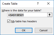
3. Press OK button.

Excel now applies formatting to your data set indicating it is now an Excel defined Table.

Search form numbers

It is now time to enter the formula, it will be automatically copied to cells below by the Excel defined Table. This is great saving us a little bit of time.

Formula in cell G2:

Make sure you use absolute cell references. The COUNTIF function counts the number of values in cell range 'Search values'!$A$2:$A$1501 that is equal to the value in column #. Here is the function syntax:

COUNTIF(range, criteria)

It returns 1 if the value in column # is found in the cell range containing conditions and 0 (zero) if not found. If there is more than one instance of a value in 'Search values'!$A$2:$A$1501 the formula may return a value greater than 1.

Filter table

The Excel defined Table lets you select which values you want to filter, there is now only 1 or 0 (zero) to choose from which is much easier to base a filter on than 1500 different conditions.

1. Press with left mouse button on the black arrow at the top in column G which is the same column you entered the formula in.
2. Make sure only 1 is selected since this indicates that the value on the same row in column # is equal to one of the 1500 conditions specified in cell range 'Search values'!$A$2:$A$1501.
   
3. Press OK button to apply the filter.

Below is a picture of the filtered Excel defined Table containing the 1500 form numbers,

12. How to use the COUNTIF function to count not blank cells

The COUNTIF function is very capable of counting non-empty values, I will show you how in this article. Excel can also highlight empty cells using Conditional formatting.

I will discuss and demonstrate the limitations of using the COUNTIF function and other equivalent functions that you also can use.

12.1. Count not blank cells - COUNTIF function

Column B above has a few blank cells, they are in fact completely empty.

Formula in cell D3:

The first argument in the COUNTIF function is the cell range where you want to count matching cells to a specific value, the second argument is the value you want to count.

COUNTIF(range, criteria)

In this case, it is "<>" meaning not equal to and then nothing, so the COUNTIF function counts the number of cells that are not equal to nothing. In other words, cells that are not empty.

Back to top

12.2. Count not blank cells - COUNTA function

The COUNTA function is even easier to use, you don't need to enter more than the cell range in one argument. The COUNTA function is designed to count non-empty cells.

COUNTA(value1, [value2], ...)

Formula in cell D4:

Back to top

12.3. COUNTIF and COUNTA function return unexpected results

There are, however, situations where the COUNTIF and COUNTA function return unexpected results if you are not aware of how they work.

There are blank cells in column C, shown in the picture above, that look empty but they are not. Column D shows what they actually contain and column E shows the character length of the content.

Cell C5 and C9 contain a formula that returns a blank, both the COUNTIF and the COUNTA function count those cells as non-empty.

Cell C8 has two space characters and cell C12 has one space character, column E reveals their existence by counting character length. The COUNTIF and the COUNTA function count those cells as non-empty as well.

Back to top

12.4. Count not blank cells - SUMPRODUCT function

The following formula counts all non-empty values in cell range C3:C13 except formulas that return nothing. It checks if the values in cell range C3:C13 are not equal to nothing.

Formula in cell B16:

Back to top

12.4.1 Explaining formula in cell B16

Step 1 - Check if cells are not empty

In this case, the logical expression counts cells that contain space characters but not formulas that return nothing.

The less than and the greater than characters are logical operators, the result are always boolean values.

C3:C13<>""

returns

{TRUE; TRUE; FALSE; TRUE; TRUE; TRUE; FALSE; TRUE; TRUE; TRUE; TRUE}

Step 2 - Convert boolean values

The SUMPRODUCT function can't sum boolean values, we need to multiply with one to create an array containing 0's (zero) and 1's.

They are their numerical equivalents:
True = 1
FALSE = 0 (zero)

(C3:C13<>"")*1

returns

{1; 1; 0; 1; 1; 1; 0; 1; 1; 1; 1}

Step 3 - Sum numbers

Why use the SUMPRODUCT function and not the SUM function? The SUMPRODUCT function can perform calculations in the arguments without the need to enter the formula as an array formula.

Array formulas are great but if possible avoid as much as you can. Excel 365 users don't have this problem, dynamic array formulas are entered as regular formulas.

SUMPRODUCT((C3:C13<>"")*1)

returns 9 in cell B16.

Back to top

12.5. Regard formulas that return nothing to be blank and space characters to also be blank

The formula above in cell C16 counts only non-empty values, it considers formulas that return nothing to be blank and space characters to also be blank. This is made possible by the TRIM function that removes leading and ending space characters.

Back to top

12.5.1 Explaining formula in cell B16

Step 1 - Remove space characters

TRIM(C3:C13)

returns

{"Green"; "Blue"; ""; "Red"; "Cyan"; ""; ""; "Yellow"; "Orange"; ""; "Brown"}

Step 2 - Identify not blank cells

TRIM(C3:C13)<>""

returns

{TRUE; TRUE; FALSE; ... ; TRUE}

Step 3 - Multiply with 1

TRIM(C3:C13)<>"")*1

returns

{1; 1; 0; ...; 1}

Step 4 - Sum numbers in array

SUMPRODUCT((TRIM(C3:C13)<>"")*1)

becomes

SUMPRODUCT({1; 1; 0; 1; 1; 0; 0; 1; 1; 0; 1})

and returns 7.

Back to top

13. Function not working

The COUNTIF function returns

• #SPILL! error if the destinations cells are not empty.
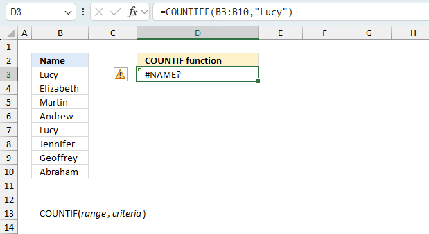
• #NAME? error if you misspell the function name.

13.1 Troubleshooting the error value

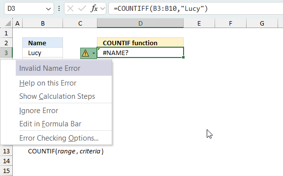
When you encounter an error value in a cell a warning symbol appears, displayed in the image above. Press with mouse on it to see a pop-up menu that lets you get more information about the error.

1. The first line describes the error if you press with left mouse button on it.
2. The second line opens a pane that explains the error in greater detail.
3. The third line takes you to the "Evaluate Formula" tool, a dialog box appears allowing you to examine the formula in greater detail.
4. This line lets you ignore the error value meaning the warning icon disappears, however, the error is still in the cell.
5. The fifth line lets you edit the formula in the Formula bar.
6. The sixth line opens the Excel settings so you can adjust the Error Checking Options.

Here are a few of the most common Excel errors you may encounter.

#NULL error - This error occurs most often if you by mistake use a space character in a formula where it shouldn't be. Excel interprets a space character as an intersection operator. If the ranges don't intersect an #NULL error is returned. The #NULL! error occurs when a formula attempts to calculate the intersection of two ranges that do not actually intersect. This can happen when the wrong range operator is used in the formula, or when the intersection operator (represented by a space character) is used between two ranges that do not overlap. To fix this error double check that the ranges referenced in the formula that use the intersection operator actually have cells in common.

#SPILL error - The #SPILL! error occurs only in version Excel 365 and is caused by a dynamic array being to large, meaning there are cells below and/or to the right that are not empty. This prevents the dynamic array formula expanding into new empty cells.

#DIV/0 error - This error happens if you try to divide a number by 0 (zero) or a value that equates to zero which is not possible mathematically.

#VALUE error - The #VALUE error occurs when a formula has a value that is of the wrong data type. Such as text where a number is expected or when dates are evaluated as text.

#REF error - The #REF error happens when a cell reference is invalid. This can happen if a cell is deleted that is referenced by a formula.

#NAME error - The #NAME error happens if you misspelled a function or a named range.

#NUM error - The #NUM error shows up when you try to use invalid numeric values in formulas, like square root of a negative number.

#N/A error - The #N/A error happens when a value is not available for a formula or found in a given cell range, for example in the VLOOKUP or MATCH functions.

#GETTING_DATA error - The #GETTING_DATA error shows while external sources are loading, this can indicate a delay in fetching the data or that the external source is unavailable right now.

13.2 The formula returns an unexpected value

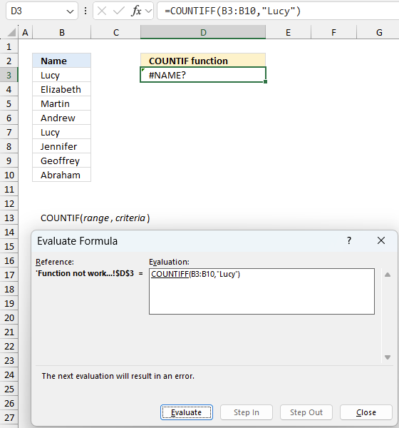
To understand why a formula returns an unexpected value we need to examine the calculations steps in detail. Luckily, Excel has a tool that is really handy in these situations. Here is how to troubleshoot a formula:

1. Select the cell containing the formula you want to examine in detail.
2. Go to tab “Formulas” on the ribbon.
3. Press with left mouse button on "Evaluate Formula" button. A dialog box appears.
   The formula appears in a white field inside the dialog box. Underlined expressions are calculations being processed in the next step. The italicized expression is the most recent result. The buttons at the bottom of the dialog box allows you to evaluate the formula in smaller calculations which you control.
4. Press with left mouse button on the "Evaluate" button located at the bottom of the dialog box to process the underlined expression.
5. Repeat pressing the "Evaluate" button until you have seen all calculations step by step. This allows you to examine the formula in greater detail and hopefully find the culprit.
6. Press "Close" button to dismiss the dialog box.

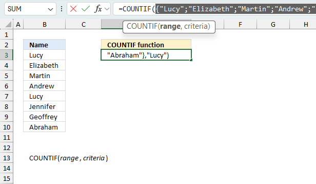
There is also another way to debug formulas using the function key F9. F9 is especially useful if you have a feeling that a specific part of the formula is the issue, this makes it faster than the "Evaluate Formula" tool since you don't need to go through all calculations to find the issue.

1. Enter Edit mode: Double-press with left mouse button on the cell or press F2 to enter Edit mode for the formula.
2. Select part of the formula: Highlight the specific part of the formula you want to evaluate. You can select and evaluate any part of the formula that could work as a standalone formula.
3. Press F9: This will calculate and display the result of just that selected portion.
4. Evaluate step-by-step: You can select and evaluate different parts of the formula to see intermediate results.
5. Check for errors: This allows you to pinpoint which part of a complex formula may be causing an error.

The image above shows cell reference B3:B10 converted to hard-coded value using the F9 key.

Tips!

• View actual values: Selecting a cell reference and pressing F9 will show the actual values in those cells.
• Exit safely: Press Esc to exit Edit mode without changing the formula. Don't press Enter, as that would replace the formula part with the calculated value.
• Full recalculation: Pressing F9 outside of Edit mode will recalculate all formulas in the workbook.

Remember to be careful not to accidentally overwrite parts of your formula when using F9. Always exit with Esc rather than Enter to preserve the original formula. However, if you make a mistake overwriting the formula it is not the end of the world. You can “undo” the action by pressing keyboard shortcut keys CTRL + z or pressing the “Undo” button

13.3 Other errors

Floating-point arithmetic may give inaccurate results in Excel - Article

Floating-point errors are usually very small, often beyond the 15th decimal place, and in most cases don't affect calculations significantly.

'COUNTIF' function examples

Functions in 'Statistical' category

The COUNTIF function function is one of 73 functions in the 'Statistical' category.

Excel function categories

Excel categories

Comments (7)