How to use the MATCH function
What is the MATCH function?
The MATCH function returns the relative position of an item in an array or cell reference that matches a specified value in a specific order.
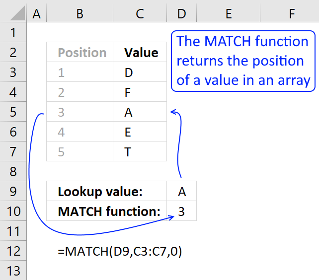
The image above shows a formula in cell D10 that searches for value "A" in cell range C3:C7 and finds an exact match in cell C5. The relative position of C5 in cell range C3:C7 is 3, shown in column B.
The MATCH function is probably one of the most used Excel functions, it is more versatile combined with the INDEX function than the VLOOKUP function. Excel 365 has newer versions of MATCH and VLOOKUP named XMATCH and XVLOOKUP respectively that are improved versions in terms of functionality and error handling.
Table of Contents
- Syntax
- Arguments
- Lookup_array in ascending order
- Lookup_array in any order
- Lookup_array in descending order
- How to use the MATCH function in an array formula
- How to do a partial match - wildcard character
- Match cell that ends with the condition
- Match cell that begins with the condition
- Match cell that contains a given string
- Match cell that begins with a specific string and ends with another string - any number of characters in between
- Match cell that begins with string and ends with another string - a single character in between
- VBA Example
- How to do a case sensitive match
- Function not working
- Get Excel *.xlsx file
1. Syntax
MATCH(lookup_value, lookup_array, [match_type])
2. Arguments
| lookup_value | Required. Is the value you use to find the value you want in the array, a number, text or logical value, or a reference to one of these. |
| lookup_array | Required. Is a contiguous range of cells containing possible lookup values, an array of values, or a reference to an array. |
| [match_type] | Optional. How to match, a number -1,0,1. If omitted default value is number 1. |
match_type
| -1 | Finds the largest value that is less than or equal to lookup_value. Lookup_array must be in ascending order. |
| 0 | Finds the value that is exactly equal to lookup_value. Lookup_array can be in any order |
| 1 | Finds the smallest value that is greater than or equal to lookup_value. Lookup_array must be sorted in a descending order |
Be careful with the third argument [match_type], remember to use 0 (zero) in the third argument if you want to find an exact match which you almost always want to.
If you don't use 0 (zero) in the third argument, the values in the lookup_array argument must be sorted in an ascending or descending order based on the lookup_array number you choose.
2.1 Comments
- The lookup_array must be a one dimensional horizontal or vertical cell range
- The lookup_value can also be an array, one or two dimensional. (array formula)
- The lookup_array can be one value. (array formula)
- You can use other Excel functions in the lookup_value argument.
- You can use other Excel functions in the lookup_array argument as long as they return a one-dimensional array.
- I use match_type = 0 almost all the time.
Below are examples demonstrating what the formula returns using different arguments.
3. Lookup_array in ascending order
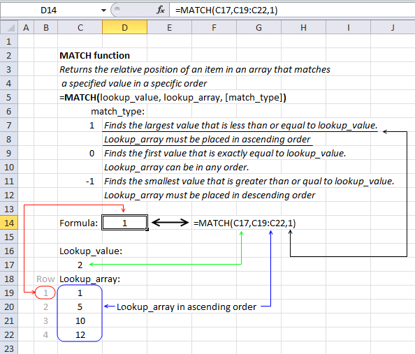
This example shows what happens and what is required if you use 1 as the [match_type] argument. Cell range C19:C21 har numbers sorted in an ascending order, which is required to get reliable results.
In this setup, the MATCH function finds the largest value that is less or equal to the lookup_value. You can use text values as well, however, make sure they are sorted in ascending order.
becomes
MATCH(2, {1; 5; 10; 12}, 1)
{1; 5; 10; 12} is an array of values separated by semicolons which means they are located in a row each.
[Match_type] 1 - Find the largest value {1; 5; 10; 12} that is less or equal to lookup_value which is 2.
MATCH(2, {1; 5; 10; 12},1)
There is only one value that is less or equal to the lookup value and that number is 1. The relative position of number 1 in array {1; 5; 10; 12} is 1. 1 is returned in cell D14.
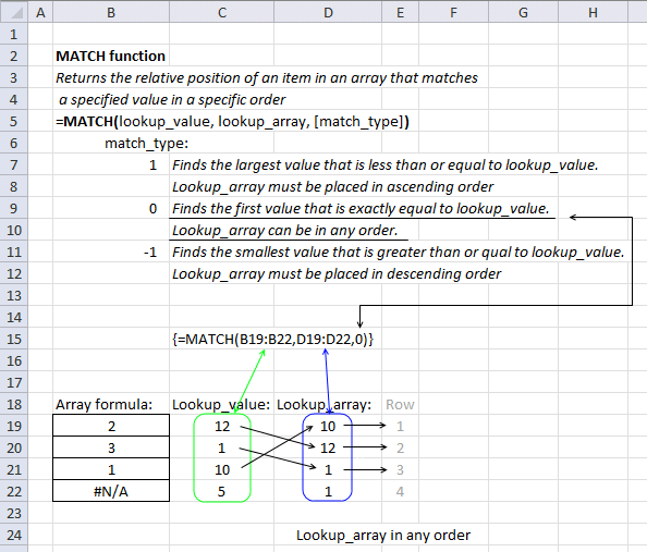
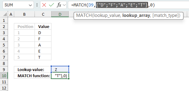
4. Example 2 - Lookup_array in any order
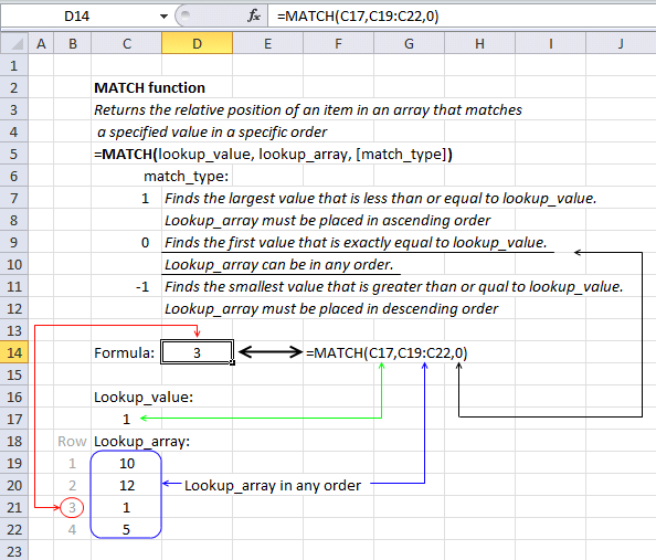
This setup is what I recommend using and is what I am using myself the most. [match_type] is 0 (zero) which allows you to have the lookup_array in any order you want.
The image above demonstrates the following formula in cell D14:
The first argument (lookup_value) is in cell C17, and the second argument (lookup_array) is in cell range C19:C22.
=MATCH(C17, C19:C21,0)
becomes
MATCH(1, {10; 12; 1; 5},0)
{10; 12; 1; 5} is an array of values separated by semicolons which means they are located in a row each.
MATCH(1, {10; 12; 1; 5},0)
Match_type 1 - Find the first value {10; 12; 1; 5} that is exactly equal to lookup_value (1)
MATCH(1, {10; 12; 1; 5},0)
The relative position of number 1 in array {10; 12; 1; 5} is 3. 3 is returned in cell D14.
5. Lookup_array in descending order
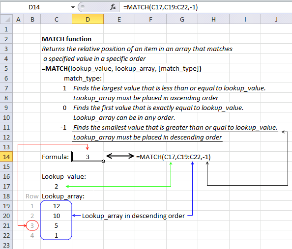
The following formula has -1 as the third argument [match_type], the lookup_array must be sorted in descending order for this setup to work.
In this case, the MATCH function finds a value in cell range C19:C22 that is larger than or equal to the lookup_value which is specified in cell C17.
becomes
MATCH(2, {12; 10; 5; 1},-1)
Match_type 1 - Find the smallest value {12; 10; 5; 1} that is greater than or equal to lookup_value (2)
MATCH(2, {12; 10; 5; 1},-1)
The relative position of number 5 in the following array {12; 10; 5; 1} is 3. 3 is returned in cell D14.
6. How to use the MATCH function in an array formula
This example demonstrates what happens if you use multiple values in the first argument lookup_value. The MATCH function returns an array of values and you are required to enter the formula as an array formula.
- Select cell range B19:B22.
- Copy the formula below and paste to cell or formula bar.
- Press and hold CTRL + SHIFT simultaneously.
- Press Enter once.
Excel adds curly brackets to the formula automatically, don't enter these characters yourself.
becomes
MATCH({12;1;10;5}, {10; 12; 1; 1},0)
Match_type 0 (zero) finds the first value {10; 12; 1; 1} that is exactly equal to lookup_value {12;1;10;5}
Lookup value 12 is the second value in the lookup_array {10; 12; 1; 1}.
Lookup value 1 is the third value in the lookup_array {10; 12; 1; 1}.
Lookup value 10 is the first value in the lookup_array {10; 12; 1; 1}.
Lookup value 5 is not found in the lookup_array {10; 12; 1; 1}.
{2; 3; 1; #N/A} is returned in cell range B19:B22.
Update!

Dynamic arrays were recently introduced to Excel 365 subscribers, they are different from regular array formulas. You don't need to enter the formula as an array formula, simply enter them as a regular formula.
Excel knows that the formula returns multiple values and extends the selection automatically, this is called spilled array behavior.

Excel returns a #SPILL! error in case there are values in cells below that prevent all array values to be displayed.
7. How to do a partial match - Wildcard characters

The asterisk character allows you to perform wilcard searches, it represents 0 (zero) to any number of characters. If this is unclear then check out the examples below.
7.1 Match cell that ends with condition
The formula in cell F3 looks for values in cell range C3:C8 that match any character and then ends with an a. No cell value in cell range C3:C8 matches that condition so the function returns #N/A error.
The formula in cell F4 is similar to cell F3 but it ends with a capital letter A. No values match that condition either and the formula returns a #N/A! error which means that the value is not available.
Formula in cell F10:
Cell E10 contains "*car" which matches the first value in cell range C3:C8, remember that the asterisk also matches no character. The formula returns 1.
7.2 Match cell that begins with condition
The next formula looks for a value that starts with an r and can contain any number of characters after that. Cell E5 contains r*.
Formula in cell F5:
The formula returns 5 which is the relative position of value "rocket" in cell range C3:C8, note that the condition would also have matched value "Rocket" and "r" and "R". The asterisk means no character up to any number of any character.
7.3 Match cell that contains string
Formula in cell F6:
The formula in cell F6 looks for a value that matches *o* which means any number of characters before and after o. The first value that matches that condition is found in position 2 which is "boat", however, there are more values that match. Value "rocket" would have matched the condition but the MATCH function returns only the number of the first value found in cell range C3:C8.
7.4 Match cell that begins with string and ends with another string - any number of characters in between
Formula in cell F7:
Cell E7 contains b*e which means that the value must begin with a b or B and must end with a e or E. Only one value matches that condition which is "bike". 7 is returned in cell F7.
7.5 Match cell that begins with string and ends with another string - a single character in between
The question mark character is different than the asterisk character, it matches only a single character.
Formula in cell F8:
Cell E8 contains b?e and the MATCH function cant find a value in cell range C3:C8 that starts with a "b", matches any single character, and ends with an "e".
Value "bike" has two characters between b and e. The formula returns #N/A! in cell F8.
Formula in cell F9:
Cell E9 contains "b?ke" and matches cell C6 which is the last value in cell range C3:C8. The formula returns 6.
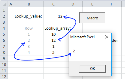
8. VBA Example
The following macro uses the MATCH function to find the position of the lookup value in cell range C5:C8. It then displays a message box containing that position.
8.1 VBA code
Sub VBA_MATCH()
MsgBox Application.WorksheetFunction.Match(Range("C2"), Range("C5:C8"), 0)
End Sub
9. How to do a case sensitive match

The formulas in column F perform a case-sensitive match, the lookup values are in column E and the lookup array is in cell range C3:C8.
Array formula in cell F4:
The result is a number representing the position of the lookup value in the lookup array.
9.1 Explaining formula in cell F4
Step 1 - Case sensitive comparison
The EXACT function performs a case-sensitive comparison. The result is a boolean value TRUE or FALSE.
EXACT(E4,$C$3:$C$8)
becomes
EXACT("TRAIN",{"Car";"boat";"Train";"airplane";"TRAIN";"bike"})
and returns
{FALSE; FALSE; FALSE; FALSE; TRUE; FALSE}.
Step 2 - Match boolean value TRUE
MATCH(TRUE, EXACT(E4, $C$3:$C$8), 0)
becomes
MATCH(TRUE, {FALSE; FALSE; FALSE; FALSE; TRUE; FALSE}, 0)
and returns 5 in cell F4.
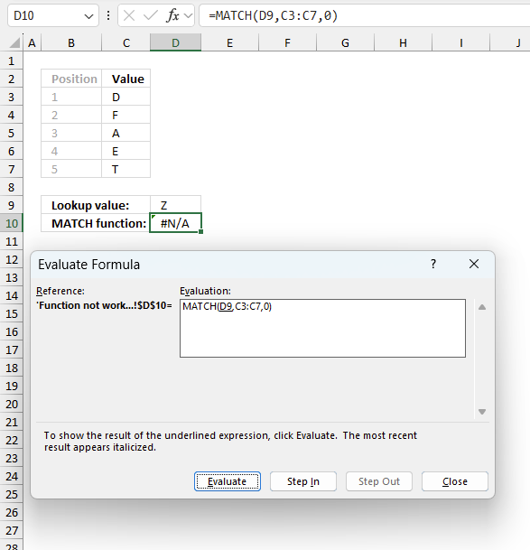
10. Function not working
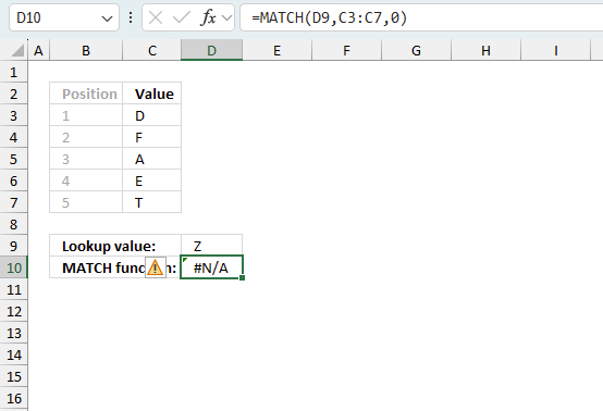
The MATCH function returns
- #N/A error if the lookup value is not found in the lookup array.
- #NAME? error if you misspell the function name.
- propagates errors, meaning that if the input contains an error (e.g., #VALUE!, #REF!), the function will return the same error.
10.1 Troubleshooting the error value
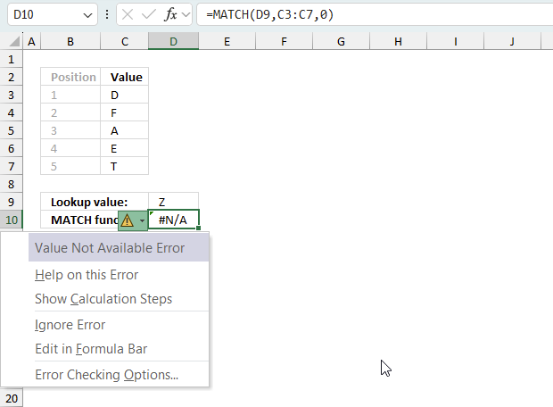
When you encounter an error value in a cell a warning symbol appears, displayed in the image above. Press with mouse on it to see a pop-up menu that lets you get more information about the error.
- The first line describes the error if you press with left mouse button on it.
- The second line opens a pane that explains the error in greater detail.
- The third line takes you to the "Evaluate Formula" tool, a dialog box appears allowing you to examine the formula in greater detail.
- This line lets you ignore the error value meaning the warning icon disappears, however, the error is still in the cell.
- The fifth line lets you edit the formula in the Formula bar.
- The sixth line opens the Excel settings so you can adjust the Error Checking Options.
Here are a few of the most common Excel errors you may encounter.
#NULL error - This error occurs most often if you by mistake use a space character in a formula where it shouldn't be. Excel interprets a space character as an intersection operator. If the ranges don't intersect an #NULL error is returned. The #NULL! error occurs when a formula attempts to calculate the intersection of two ranges that do not actually intersect. This can happen when the wrong range operator is used in the formula, or when the intersection operator (represented by a space character) is used between two ranges that do not overlap. To fix this error double check that the ranges referenced in the formula that use the intersection operator actually have cells in common.
#SPILL error - The #SPILL! error occurs only in version Excel 365 and is caused by a dynamic array being to large, meaning there are cells below and/or to the right that are not empty. This prevents the dynamic array formula expanding into new empty cells.
#DIV/0 error - This error happens if you try to divide a number by 0 (zero) or a value that equates to zero which is not possible mathematically.
#VALUE error - The #VALUE error occurs when a formula has a value that is of the wrong data type. Such as text where a number is expected or when dates are evaluated as text.
#REF error - The #REF error happens when a cell reference is invalid. This can happen if a cell is deleted that is referenced by a formula.
#NAME error - The #NAME error happens if you misspelled a function or a named range.
#NUM error - The #NUM error shows up when you try to use invalid numeric values in formulas, like square root of a negative number.
#N/A error - The #N/A error happens when a value is not available for a formula or found in a given cell range, for example in the VLOOKUP or MATCH functions.
#GETTING_DATA error - The #GETTING_DATA error shows while external sources are loading, this can indicate a delay in fetching the data or that the external source is unavailable right now.
10.2 The formula returns an unexpected value
To understand why a formula returns an unexpected value we need to examine the calculations steps in detail. Luckily, Excel has a tool that is really handy in these situations. Here is how to troubleshoot a formula:
- Select the cell containing the formula you want to examine in detail.
- Go to tab “Formulas” on the ribbon.
- Press with left mouse button on "Evaluate Formula" button. A dialog box appears.
The formula appears in a white field inside the dialog box. Underlined expressions are calculations being processed in the next step. The italicized expression is the most recent result. The buttons at the bottom of the dialog box allows you to evaluate the formula in smaller calculations which you control. - Press with left mouse button on the "Evaluate" button located at the bottom of the dialog box to process the underlined expression.
- Repeat pressing the "Evaluate" button until you have seen all calculations step by step. This allows you to examine the formula in greater detail and hopefully find the culprit.
- Press "Close" button to dismiss the dialog box.
There is also another way to debug formulas using the function key F9. F9 is especially useful if you have a feeling that a specific part of the formula is the issue, this makes it faster than the "Evaluate Formula" tool since you don't need to go through all calculations to find the issue..
- Enter Edit mode: Double-press with left mouse button on the cell or press F2 to enter Edit mode for the formula.
- Select part of the formula: Highlight the specific part of the formula you want to evaluate. You can select and evaluate any part of the formula that could work as a standalone formula.
- Press F9: This will calculate and display the result of just that selected portion.
- Evaluate step-by-step: You can select and evaluate different parts of the formula to see intermediate results.
- Check for errors: This allows you to pinpoint which part of a complex formula may be causing an error.
The image above shows cell reference C3:C7 converted to hard-coded value using the F9 key. The MATCH function requires a lookup value that exists in the lookup array which is not the case in this example. We have found what is wrong with the formula.
Tips!
- View actual values: Selecting a cell reference and pressing F9 will show the actual values in those cells.
- Exit safely: Press Esc to exit Edit mode without changing the formula. Don't press Enter, as that would replace the formula part with the calculated value.
- Full recalculation: Pressing F9 outside of Edit mode will recalculate all formulas in the workbook.
Remember to be careful not to accidentally overwrite parts of your formula when using F9. Always exit with Esc rather than Enter to preserve the original formula. However, if you make a mistake overwriting the formula it is not the end of the world. You can “undo” the action by pressing keyboard shortcut keys CTRL + z or pressing the “Undo” button
10.3 Other errors
Floating-point arithmetic may give inaccurate results in Excel - Article
Floating-point errors are usually very small, often beyond the 15th decimal place, and in most cases don't affect calculations significantly.
MATCH function links
'MATCH' function examples

First, let me explain the difference between unique values and unique distinct values, it is important you know the difference […]

This post explains how to lookup a value and return multiple values. No array formula required.

Array formulas allows you to do advanced calculations not possible with regular formulas.
Functions in 'Lookup and reference' category
The MATCH function function is one of 25 functions in the 'Lookup and reference' category.
Excel function categories
Excel categories
12 Responses to “How to use the MATCH function”
Leave a Reply
How to comment
How to add a formula to your comment
<code>Insert your formula here.</code>
Convert less than and larger than signs
Use html character entities instead of less than and larger than signs.
< becomes < and > becomes >
How to add VBA code to your comment
[vb 1="vbnet" language=","]
Put your VBA code here.
[/vb]
How to add a picture to your comment:
Upload picture to postimage.org or imgur
Paste image link to your comment.
[...] MATCH(lookup_value;lookup_array; [match_type]) Returns the relative position of an item in an array that matches a specified value [...]
Oscar,
You might want to read the comments of the below post to see couple of more interesting uses of the MATCH Function
https://fastexcel.wordpress.com/2013/02/27/speedtools-avlookup2-memlookup-versus-vlookup-performance-power-and-ease-of-use-shootout-part-1/#comments
sam,
Very interesting comment! I never thought of that.
Thank you for commenting!
Respected sir,
You solved one of my excel related problem some months back. This time I have another problem. This time I have some fields as below:
Capacity City books Big_Boxes small_Boxes Total
90 Kanpur 400 4 1 5
Lucknow 690 7 1 8
Jhansi 240 2 1 3
Allahabad 20 0 1 1
Total 17
Now, I have to generate slips to paste on boxes which are to be despatched:
City: Kanpur
No_of_Text_Books in this Box 90 Box No.1
Total_No._of_Books 400 in 5 Boxes
These slips are to be generated till end. Please help me.
neeraj kumar,
Formula in cell A10:
Formula in cell A11:
Get the Excel *.xlsx file
neeraj-kumar.xlsx
[…] MATCH(lookup_value, lookup_array, [match_type] Returns the relative position of an item in an array that matches a specified value […]
[…] MATCH(lookup_value, lookup_array, [match_type] Returns the relative position of an item in an array that matches a specified value. […]
[…] Match function […]
[…] and returns 2. Read more about MATCH function. […]
[…] MATCH(lookup_value;lookup_array, [match_type]) Returns the relative position of an item in an array that matches a specified value […]
[…] MATCH(lookup_value,lookup_array, [match_type]) Returns the relative position of an item in an array that matches a specified value […]