How to use the MIN function
What is the MIN function?
The MIN function allows you to retrieve the smallest number in a cell range.
When is the MIN function useful in statistics?
The MIN function allows you to find the minimum or lowest value in a set of data points. This can be helpful when you want to identify outliers or extreme values in your dataset.
The range of a dataset is the difference between the maximum and minimum values. You can use the MIN function in combination with the MAX function to calculate the range which is a measure of the spread of the data.
Table of Contents
1. Syntax
MIN(number1, [number2], ...)
2. Arguments
| Argument | Text |
| number1 | You need at least one argument. Required. |
| [number2] | Up to 254 arguments are possible. Optional. |
3. Example 1
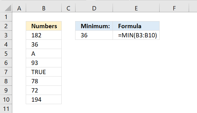
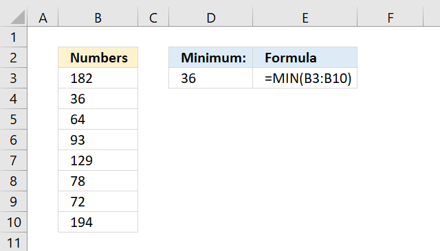
The image above shows the MIN function in cell D3, Cell range B3:B10 contains random text, numbers, and boolean values. Here is the data in cell range B3:B10:
| 182 |
| 36 |
| A |
| 93 |
| TRUE |
| 78 |
| 72 |
| 194 |
The MIN function ignores text and boolean values, however not errors.
Formula in cell E3:
Arguments can be constants, named ranges, cell references, and arrays.
MIN(B3:B10) becomes
MIN({182; 36; "A"; 93; TRUE; 78; 72; 194}) and returns 36. Number 36 is the smallest number in the data set.
4. Example 2 - ignore zero

The image above demonstrates a formula that extracts the smallest number in a given cell range also ignoring zeros. Cell range B2:B10 contains the following data:
| Numbers |
| 182 |
| 36 |
| 0 |
| 93 |
| 0 |
| 78 |
| 72 |
| 194 |
Note that cells B5 and B7 contains 0 (zero), the formula below removes zeros from the calculation and replaces them with a blank that the MIN function ignores.
Array formula in cell D3:
The smallest value of this data set ignoring zeros: {182;36;0;93;0;78;72;194} is 36.
4.1 How to enter an array formula

- Copy the array formula above.
- Double press with the left mouse button on cell D3, a prompt appears.
- Paste it to cell D3, shortcut keys are CTRL + v.
- Press and hold CTRL + SHIFT keys simultaneously.
- Press Enter once.
- Release all keys.
The formula bar shows a beginning and ending curly bracket, don't enter these characters yourself.
They appear automatically if you followed the above steps.
4.2 Explaining formula
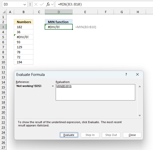
The Evaluate Formula tool is located on the Formulas tab in the Ribbon. It is a useful feature that allows you to step through and evaluate complex formulas to understand how the calculation is being performed and identify any errors or issues. The following steps shows these detailed evaluations for the formula above.
Step 1 - Find numbers not equal to zero
The less than and larger than signs combined evaluates to not equal to, the result is a boolean value TRUE or FALSE.
B3:B10<>0
becomes
{182; 36; 0; 93; 0; 78; 72; 194}<>0
and returns
{TRUE; TRUE; FALSE; TRUE; FALSE; TRUE; TRUE; TRUE}.
Step 2 - Replace TRUE with nothing
The IF function returns one value if the logical test is TRUE and another value if the logical test is FALSE.
IF(logical_test, [value_if_true], [value_if_false])
IF(B3:B10<>0, B3:B10, "")
becomes
IF({TRUE; TRUE; FALSE; TRUE; FALSE; TRUE; TRUE; TRUE}, B3:B10, "")
becomes
IF({TRUE; TRUE; FALSE; TRUE; FALSE; TRUE; TRUE; TRUE}, {182; 36; 0; 93; 0; 78; 72; 194}, "")
and returns {182; 36; ""; 93; ""; 78; 72; 194}.
Step 3 - Extract smallest number in array
MIN(IF(B3:B10<>0, B3:B10, ""))
becomes
MIN({182; 36; ""; 93; ""; 78; 72; 194})
and returns 36.
5. Example 3 - returns 0 (zero)

The image above shows a scenario where the MIN function returns zero and the data source contains no zeros, at least, that is what it looks like.
Formula in cell D3:
Cell B3:B10 contains blank cells but when we check the cell formatting dialog box, zeros have been hidden. See the image below.

Here is how to check if zeros are hidden.
- Select your data. Cell range B3:B10 in this example.
- Press CTRL + 1 to open the "Format Cells" dialog box.
- Select category "General".
- Press with the left mouse button on the "OK" button to apply changes.

Check the Excel options if this is not working for you. Here is how to do that in Excel 365:
- Press with the left mouse button on tab "File" on the ribbon.
- Press with left mouse button on "Options".
- Go to "Advanced", see the image below.

- Scroll down until you find "Show a zero in cells that have zero value". Make sure the checkbox is enabled.
- Press with the left mouse button on the "OK" button to apply changes.
Check the next section if this is also not a solution for you.
6. Function not working

This example demonstrates numbers stored as text may make the MIN function return 0 (zero). Numbers stored as text are left-aligned (default), a green arrow in the top left corner is an indication of numbers stored as text.
Formula in cell D3:
Here is how to convert numbers stored as text.
- Select the data, this is cell range B3:B10 in the example above.

- An "exclamation" sign appears.
- Press with left mouse button on the "Exclamation" sign to open a context menu.

- Press with left mouse button on "Convert to Number".

The MIN function is now working.
6.1 Troubleshooting the error value
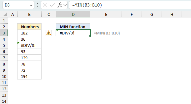
When you encounter an error value in a cell a warning symbol appears, displayed in the image above. Press with mouse on it to see a pop-up menu that lets you get more information about the error.
- The first line describes the error if you press with left mouse button on it.
- The second line opens a pane that explains the error in greater detail.
- The third line takes you to the "Evaluate Formula" tool, a dialog box appears allowing you to examine the formula in greater detail.
- This line lets you ignore the error value meaning the warning icon disappears, however, the error is still in the cell.
- The fifth line lets you edit the formula in the Formula bar.
- The sixth line opens the Excel settings so you can adjust the Error Checking Options.
Here are a few of the most common Excel errors you may encounter.
#NULL error - This error occurs most often if you by mistake use a space character in a formula where it shouldn't be. Excel interprets a space character as an intersection operator. If the ranges don't intersect an #NULL error is returned. The #NULL! error occurs when a formula attempts to calculate the intersection of two ranges that do not actually intersect. This can happen when the wrong range operator is used in the formula, or when the intersection operator (represented by a space character) is used between two ranges that do not overlap. To fix this error double check that the ranges referenced in the formula that use the intersection operator actually have cells in common.
#SPILL error - The #SPILL! error occurs only in version Excel 365 and is caused by a dynamic array being to large, meaning there are cells below and/or to the right that are not empty. This prevents the dynamic array formula expanding into new empty cells.
#DIV/0 error - This error happens if you try to divide a number by 0 (zero) or a value that equates to zero which is not possible mathematically.
#VALUE error - The #VALUE error occurs when a formula has a value that is of the wrong data type. Such as text where a number is expected or when dates are evaluated as text.
#REF error - The #REF error happens when a cell reference is invalid. This can happen if a cell is deleted that is referenced by a formula.
#NAME error - The #NAME error happens if you misspelled a function or a named range.
#NUM error - The #NUM error shows up when you try to use invalid numeric values in formulas, like square root of a negative number.
#N/A error - The #N/A error happens when a value is not available for a formula or found in a given cell range, for example in the VLOOKUP or MATCH functions.
#GETTING_DATA error - The #GETTING_DATA error shows while external sources are loading, this can indicate a delay in fetching the data or that the external source is unavailable right now.
6.2 The formula returns an unexpected value
To understand why a formula returns an unexpected value we need to examine the calculations steps in detail. Luckily, Excel has a tool that is really handy in these situations. Here is how to troubleshoot a formula:
- Select the cell containing the formula you want to examine in detail.
- Go to tab “Formulas” on the ribbon.
- Press with left mouse button on "Evaluate Formula" button. A dialog box appears.
The formula appears in a white field inside the dialog box. Underlined expressions are calculations being processed in the next step. The italicized expression is the most recent result. The buttons at the bottom of the dialog box allows you to evaluate the formula in smaller calculations which you control. - Press with left mouse button on the "Evaluate" button located at the bottom of the dialog box to process the underlined expression.
- Repeat pressing the "Evaluate" button until you have seen all calculations step by step. This allows you to examine the formula in greater detail and hopefully find the culprit.
- Press "Close" button to dismiss the dialog box.
There is also another way to debug formulas using the function key F9. F9 is especially useful if you have a feeling that a specific part of the formula is the issue, this makes it faster than the "Evaluate Formula" tool since you don't need to go through all calculations to find the issue..
- Enter Edit mode: Double-press with left mouse button on the cell or press F2 to enter Edit mode for the formula.
- Select part of the formula: Highlight the specific part of the formula you want to evaluate. You can select and evaluate any part of the formula that could work as a standalone formula.
- Press F9: This will calculate and display the result of just that selected portion.
- Evaluate step-by-step: You can select and evaluate different parts of the formula to see intermediate results.
- Check for errors: This allows you to pinpoint which part of a complex formula may be causing an error.
The image above shows cell reference B3:B10 converted to hard-coded value using the F9 key. The MIN function requires non-error values which is not the case in this example. We have found what is wrong with the formula.
Tips!
- View actual values: Selecting a cell reference and pressing F9 will show the actual values in those cells.
- Exit safely: Press Esc to exit Edit mode without changing the formula. Don't press Enter, as that would replace the formula part with the calculated value.
- Full recalculation: Pressing F9 outside of Edit mode will recalculate all formulas in the workbook.
Remember to be careful not to accidentally overwrite parts of your formula when using F9. Always exit with Esc rather than Enter to preserve the original formula. However, if you make a mistake overwriting the formula it is not the end of the world. You can “undo” the action by pressing keyboard shortcut keys CTRL + z or pressing the “Undo” button
6.3 Other errors
Floating-point arithmetic may give inaccurate results in Excel - Article
Floating-point errors are usually very small, often beyond the 15th decimal place, and in most cases don't affect calculations significantly.
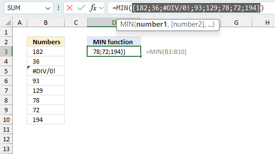
7. Example 4 - ignore errors

The formula in cell D3 extracts the smallest number in cell range B3:B10 ignoring error values. Cell range B2:B10 contains the following values:
| Numbers |
| 182 |
| 36 |
| #N/A |
| 93 |
| #DIV/0! |
| 78 |
| 72 |
| 194 |
Note that cells B5 and B7 contain error values.
Array formula in cell D3:
The smallest number in this data set: {182;36;#N/A;93;#DIV/0!;78;72;194} is 36.
7.1 Explaining formula
The Evaluate Formula tool is located on the Formulas tab in the Ribbon. It is a useful feature that allows you to step through and evaluate complex formulas to understand how the calculation is being performed and identify any errors or issues. The following steps shows these detailed evaluations for the formula above.
Step 1 - Replace error values with nothing
The IFERROR function introduced in Excel 2007 lets you handle most errors in Excel formulas.
IFERROR(value, value_if_error)
IFERROR(B3:B10,"")
becomes
IFERROR({182; 36; #N/A; 93; #DIV/0!; 78; 72; 194})
and returns
{182; 36; ""; 93; ""; 78; 72; 194}
Step 2 - Extract smallest number
MIN(IFERROR(B3:B10,""))
becomes
MIN({182; 36; ""; 93; ""; 78; 72; 194})
and returns 36.
8. Example 5 - ignoring negative numbers

This example demonstrates an array formula in cell D3 that extracts the smallest number in cell range B3:B10 if equal to or larger than zero. Cell range B3:B10 contains these values:
| Numbers |
| 182 |
| 36 |
| -5 |
| 93 |
| -11 |
| 78 |
| 72 |
| 194 |
The formula filters values larger than or equal to zero, then finds the smallest number.
Array formula in cell D3:
182, 36, -5, 93, -11, 78, 72, and 194 contains two negative values -5 and -11. IF we ignore the negative values the smallest number in the remaining group is 36 which is the value displayed in cell D3.
Explaining formula
The Evaluate Formula tool is located on the Formulas tab in the Ribbon. It is a useful feature that allows you to step through and evaluate complex formulas to understand how the calculation is being performed and identify any errors or issues. The following steps shows these detailed evaluations for the formula above.
Step 1 - Filter out negative numbers
The larger than and the equal sign lets you identify numbers larger than or equal to zero, the result is a boolean value TRUE or FALSE.
B3:B10>=0
becomes
{182; 36; -5; 93; -11; 78; 72; 194}>=0
and returns
{TRUE; TRUE; FALSE; TRUE; FALSE; TRUE; TRUE; TRUE}.
Step 2 - Replce TRUE with corresponding number
The IF function returns one value if the logical test is TRUE and another value if the logical test is FALSE.
IF(logical_test, [value_if_true], [value_if_false])
IF(B3:B10>=0, B3:B10, "")
becomes
IF({TRUE; TRUE; FALSE; TRUE; FALSE; TRUE; TRUE; TRUE}, {182; 36; -5; 93; -11; 78; 72; 194}, "")
and returns
{182; 36; ""; 93; ""; 78; 72; 194}.
Step 3 - Extract the smallest number
MIN(IF(B3:B10>=0,B3:B10,""))
becomes
MIN({182; 36; ""; 93; ""; 78; 72; 194})
and returns 36.
9. Example 6 - ignore text

The MIN function ignores text values out of the box, there is no need for you to do anything about it. The example above demonstrates two text values in cells B5 and B7, the formula in cell D3 extracts the smallest number in B3:B10 ignoring the text values. The values in cell range B3:B10 are:
| Numbers |
| 182 |
| 36 |
| A |
| 93 |
| B |
| 78 |
| 72 |
| 194 |
Formula in cell D3:
The formula in cell D3 returns 36 which is the smallest number in B3:B10.
10. Example 7 - ignore #NA error

This example demonstrates a formula that ignores #N/A error values.Cell range B3:B10 contains these values:
| Numbers |
| 182 |
| 36 |
| #N/A |
| 93 |
| #N/A |
| 78 |
| 72 |
| 194 |
Note that cells B5 and B7 contain #N/A errors.
Array formula in cell D3:
The formula ignores the #N/A errors and returns the smallest number in B3:B10 which is 36.
Explaining formula
The Evaluate Formula tool is located on the Formulas tab in the Ribbon. It is a useful feature that allows you to step through and evaluate complex formulas to understand how the calculation is being performed and identify any errors or issues. The following steps shows these detailed evaluations for the formula above.
Step 1 - Identify #N/A errors
The ISNA function returns TRUE if a given value is #N/A.
ISNA(value)
ISNA(B3:B10)
becomes
ISNA({182; 36; #N/A; 93; #N/A; 78; 72; 194})
and returns
{FALSE; FALSE; TRUE; FALSE; TRUE; FALSE; FALSE; FALSE}.
Step 2 - Replace TRUE with nothing
The IF function returns one value if the logical test is TRUE and another value if the logical test is FALSE.
IF(logical_test, [value_if_true], [value_if_false])
IF(ISNA(B3:B10), "", B3:B10)
becomes
IF({FALSE; FALSE; TRUE; FALSE; TRUE; FALSE; FALSE; FALSE}, "", B3:B10)
becomes
IF({FALSE; FALSE; TRUE; FALSE; TRUE; FALSE; FALSE; FALSE}, "", {182; 36; #N/A; 93; #N/A; 78; 72; 194})
and returns
{182; 36; ""; 93; ""; 78; 72; 194}.
Step 3 - Extract minimum number
MIN(IF(ISNA(B3:B10), "", B3:B10))
becomes
MIN({182; 36; ""; 93; ""; 78; 72; 194})
and returns 36.
'MIN' function examples

Array formulas allows you to do advanced calculations not possible with regular formulas.
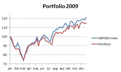
Table of Contents Compare the performance of your stock portfolio to S&P 500 Tracking a stock portfolio in Excel (auto […]
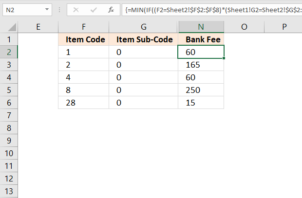
This article describes an array formula that compares values from two different columns in two worksheets twice and returns a […]
Functions in 'Statistical' category
The MIN function function is one of 73 functions in the 'Statistical' category.
Excel function categories
Excel categories
One Response to “How to use the MIN function”
Leave a Reply
How to comment
How to add a formula to your comment
<code>Insert your formula here.</code>
Convert less than and larger than signs
Use html character entities instead of less than and larger than signs.
< becomes < and > becomes >
How to add VBA code to your comment
[vb 1="vbnet" language=","]
Put your VBA code here.
[/vb]
How to add a picture to your comment:
Upload picture to postimage.org or imgur
Paste image link to your comment.
hola buen dia necesito sacar el minimo ejemplo de la columna (C5,D5,E5) ya utilice la formula =MIN(C5:E5) y no me funciona ya que en estas 3 columnas ahi filas que no tienen valor o el valor es 0 me podrias dar el informe o la formula para sacar este dato gracias..