How to use the TOCOL function

What is the TOCOL function?
The TOCOL function lets you rearrange values in 2D cell ranges to a single column.
What is TOCOL an abbreviation of?
TOCOL stands for to column.
Which Excel version is TOCOL in?
The TOCOL function is available to Excel 365 users
What category is the TOCOL function in?
The TOCOL function is in the "Array manipulation" category.
Table of Contents
1. Syntax
The TOCOL function has three arguments, the first one is required the other two are optional.
TOCOL(array, [ignore], [scan_by_col])
2. Arguments
| array | Required. The source cell range or array. Use parentheses and comma delimiter to add more arrays or cell ranges. See section 7 below for an example. |
| [ignore] | Optional. Ignore specified values. 0 - keep all values (default) 1 - ignore blanks 2 - ignore errors 3- ignore blanks and errors |
| [scan_by_col] | Optional. How the function fetches the values from the source. FALSE - by row (default). TRUE - by column. |
3. Example

The image above demonstrates how the TOCOL function rearranges the values to fit a single column, and that it is fetching values by row in its default state.
This means that the TOCOL function takes the values in cell B2:E4 row by row and transposes them so they fit a single column. For example, the first row is 89, 68, 19, and 37 and they are distributed horizontally in B2:E2,
The TOCOL function rearranges the values so they are distributed vertically like this: 89; 68; 19; 37. It the goes on to the second row and transposes those values below the first row. The blue arrows shows this beahviour in the TOCOL functions default state. You can however change this so it scans the cell range column by column instead of row by row.
Dynamic array formula in cell E4:
The TOCOL function is incredibly useful if you want to for example extract unique distinct values across multiple columns. The UNIQUE function requires an array containing values distributed vertically one by one. If not the UNIQUE function extracts unique distinct rows.
3.1 Explaining formula
Tip! You can follow the formula calculations step by step by using the "Evaluate" tool located on the Formula tab on the ribbon. This makes it easier to spot errors and understand the formula in greater detail. The following steps shows the calculations in great detail.
Step 1 - TOCOL function
TOCOL(array, [ignore], [scan_by_col])
Step 2 - Populate arguments
array - B2:E4
Step 3 - Evaluate function
TOCOL(B2:E4)
becomes
TOCOL({89, 68, 19, 37;
27, 84, 92, 63;
26, 98, 62, 100})
and returns
{89; 68; 19; 37; 27; 84; 92; 63; 26; 98; 62; 100}
4. Example - by column

The image above demonstrates how the TOCOL function rearranges the values to fit a single column. This example shows it fetching values column by column. Default value is FALSE - which means by row.
The blue arrows show that the TOCOL function is also capable of rearranging values column by column. The first column is 89, 27, 26, 68 which is also displayed in the output array in cell E4. The second column is then put below these values, this continues column by column until all columns have been scanned.
Dynamic array formula in cell E4:
The third argument lets you specify the scan state: scan_by_col or scan_by_row. TRUE means scan_by_col and FALSE means scan_by_row which is also the default state.
4.1 Explaining formula
Tip! You can follow the formula calculations step by step by using the "Evaluate" tool located on the Formula tab on the ribbon. This makes it easier to spot errors and understand the formula in greater detail. The following steps shows the calculations in great detail.
Step 1 - TOCOL function
TOCOL(array, [ignore], [scan_by_col])
Step 2 - Populate arguments
array - B2:E4
[scan_by_col]) - TRUE
Step 3 - Evaluate function
TOCOL(B2:E4, , TRUE)
becomes
TOCOL({89, 68, 19, 37;
27, 84, 92, 63;
26, 98, 62, 100})
and returns
{89; 68; 19; 37; 27; 84; 92; 63; 26; 98; 62; 100}
5. Blanks and errors

The TOCOL function can handle blanks and errors, however, you must specify that in the aruments if you want that functionality. The image above demonstrates what happens when your source data has empty values and errors. The result is an array containing a 0 (zero) located at the empty values and the error values are kept.
Dynamic array formula in cell E4:
The image below shows how to deal with blanks and error values.

You can ignore blank and error values using the second argument.
Here are all valid numbers for the second argument:
0 - keep all values (default)
1 - ignore blanks
2 - ignore errors
3- ignore blanks and errors
Dynamic array formula in cell E4:
There is an instance when this doesn't work. This happens if you use the IF function to filter specific values in the TOCOL function. Here is an example.
=TOCOL(IF(B2:E4<50,"",B2:E4), 3)
The TOCOL function can't handle blanks and errors from the IF function at all, they all show even if you use 3 in the second argument. This is kind of a disappointment, I hope Microsoft software engineers fix this issue in upcoming releases.
5.1 Explaining formula
TOCOL(array, [ignore], [scan_by_col])
TOCOL(B2:E4, 3)
becomes
TOCOL({89, 68, 19, 37;
27, 0, 92, 63;
26, 98, 62, #DIV/0!}
)
and returns
{89; 68; 19; 37; 27; 92; 63; 26; 98; 62}
6. Alternative
There are no great alternative formulas for earlier Excel versions. Here are a few links:
- Rearrange values in a cell range to a single column
- Combine cell ranges ignore blank cells
- Merge two columns
- Merge three columns into one list
7. Example - multiple cell ranges as source

You can consolidate values across worksheets if you combine the VSTACK function and the TOCOL function, the formula spills values into a single column.
The image above shows how to combine values from cell ranges B2:C3, E2:F3, and h3:I3 into a single column.
Dynamic array formula in cell B8:
The formula in cell B8 joins the three non-adjacent cell ranges vertically and then scans the resulting array row by row and rearranges the values to a single column. You can try different outcomes based on how you want the values arranged. The HSTACK function joins the cell ranges horizontally, and the third argument in the TOCOL function lets you specify how the function scans and rearranges the values in the array. The options are scan_by_row or scan_by_column.
Update! The TOCOL function accepts multiple references in the array argument. There is no need for the VSTACK function. Here is how:
The parentheses and a delimiting comma let you use multiple non-adjacent cell ranges. Note that this is done in the first argument.
7.1 Explaining formula
Tip! You can follow the formula calculations step by step by using the "Evaluate" tool located on the Formula tab on the ribbon. This makes it easier to spot errors and understand the formula in greater detail. The following steps shows the calculations in great detail.
Step 1 - Stack values from multiple sources
The VSTACK function lets you combine cell ranges or arrays, it joins data to the first blank cell at the bottom of a cell range or array.
VSTACK(array1,[array2],...)
VSTACK(B2:C3, E2:F3, h3:I3)
becomes
VSTACK({89,68;27,84}, {19,37;92,63}, {26,98;62,100})
and returns
{89,68;
27,84;
19,37;
92,63;
26,98;
62,100}
Step 2 - Rearrange values into one column
TOCOL(VSTACK(B2:C3, E2:F3, h3:I3))
becomes
TOCOL({89,68;
27,84;
19,37;
92,63;
26,98;
62,100})
and returns
{89; 68; 27; 84; 19; 37; 92; 63; 26; 98; 62; 100}
8. Extract unique distinct values from a multi-column cell range

The UNIQUE function doesn't let you extract unique distinct values if your source data has multiple columns, it will return unique distinct rows instead.
However, the TOCOL function allows you to rearrange the values to a single column array, and that lets you extract unique distinct values.
Dynamic array formula in cell B8:
The TOCOL function makes it so much easier to extract unique distinct values. The values must be arranged in a single column for the UNIQUE function to work properly.
8.1 Explaining formula
Tip! You can follow the formula calculations step by step by using the "Evaluate" tool located on the Formula tab on the ribbon. This makes it easier to spot errors and understand the formula in greater detail. The following steps shows the calculations in great detail.
Step 1 - Rearrange values
TOCOL(array, [ignore], [scan_by_col])
TOCOL(B2:G5)
returns {"Elizabeth"; "Patricia"; ... ; "Mary"}.
The column delimiting character changed from a comma to a semicolon in the array above. This means that each value is in a new row, in other words, values are rearranged to fit a single column.
Step 2 - Extract unique distinct values
The UNIQUE function is a new Excel 365 function that returns unique and unique distinct values/rows.
UNIQUE(array,[by_col],[exactly_once])
UNIQUE(TOCOL(B2:G5))
returns {"Elizabeth";"Patricia";"Jennifer";"William";"John";"Robert";"Mary";"Michael";"Linda"}.
9. Extract unique distinct values from multiple cell ranges

You can consolidate values across worksheets, rearrange values so they fit a single column, and then extract unique distinct values.
The image above shows a formula that extracts unique distinct values from three different non-adjacent cell ranges.
Dynamic array formula in cell B8:
Update!
No need to use the HSTACK function. Use the comma as a union operator, it combines multiple cell ranges.
This formula is useful for getting values across worksheets consolidated into one array, it is also dynamic meaning it changes instantly if the source ranges change.
9.1 Explaining formula
Step 1 - Rearrange values
The HSTACK function lets you combine cell ranges or arrays, it joins data to the first blank cell to the right of a cell range or array (horizontal stacking)
HSTACK(array1,[array2],...)
HSTACK(B2:C5, E2:F5, h3:I5)
returns {"Elizabeth", "Patricia", ... , "Mary"}
Step 2 - Rearrange values to one column
TOCOL(array, [ignore], [scan_by_col])
TOCOL(HSTACK(B2:C5, E2:F5, h3:I5))
returns
{"Elizabeth"; "Patricia"; ... ; "Mary"}.
Step 3 - Extract unique distinct values
The UNIQUE function is a new Excel 365 function that returns unique and unique distinct values/rows.
UNIQUE(array,[by_col],[exactly_once])
UNIQUE(TOCOL(HSTACK(B2:C5, E2:F5, h3:I5)))
returns
{"Elizabeth"; "Patricia"; "Jennifer"; "William"; "John"; "Robert"; "Mary"; "Michael"; "Linda"}.
10. Function not working
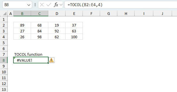
The TOCOL function returns
- #VALUE! error if the second argument is invalid.
- #NAME? error if you misspell the function name.
- propagates errors, meaning that if the input contains an error (e.g., #VALUE!, #REF!), the function will return the same error.
10.1 Troubleshooting the error value
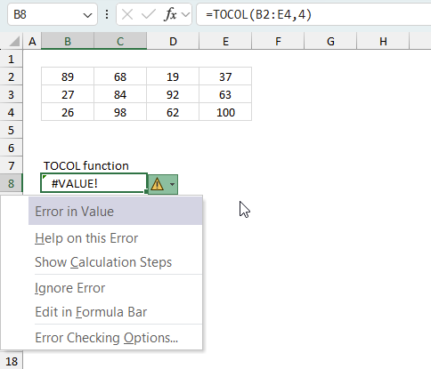
When you encounter an error value in a cell a warning symbol appears, displayed in the image above. Press with mouse on it to see a pop-up menu that lets you get more information about the error.
- The first line describes the error if you press with left mouse button on it.
- The second line opens a pane that explains the error in greater detail.
- The third line takes you to the "Evaluate Formula" tool, a dialog box appears allowing you to examine the formula in greater detail.
- This line lets you ignore the error value meaning the warning icon disappears, however, the error is still in the cell.
- The fifth line lets you edit the formula in the Formula bar.
- The sixth line opens the Excel settings so you can adjust the Error Checking Options.
Here are a few of the most common Excel errors you may encounter.
#NULL error - This error occurs most often if you by mistake use a space character in a formula where it shouldn't be. Excel interprets a space character as an intersection operator. If the ranges don't intersect an #NULL error is returned. The #NULL! error occurs when a formula attempts to calculate the intersection of two ranges that do not actually intersect. This can happen when the wrong range operator is used in the formula, or when the intersection operator (represented by a space character) is used between two ranges that do not overlap. To fix this error double check that the ranges referenced in the formula that use the intersection operator actually have cells in common.
#SPILL error - The #SPILL! error occurs only in version Excel 365 and is caused by a dynamic array being to large, meaning there are cells below and/or to the right that are not empty. This prevents the dynamic array formula expanding into new empty cells.
#DIV/0 error - This error happens if you try to divide a number by 0 (zero) or a value that equates to zero which is not possible mathematically.
#VALUE error - The #VALUE error occurs when a formula has a value that is of the wrong data type. Such as text where a number is expected or when dates are evaluated as text.
#REF error - The #REF error happens when a cell reference is invalid. This can happen if a cell is deleted that is referenced by a formula.
#NAME error - The #NAME error happens if you misspelled a function or a named range.
#NUM error - The #NUM error shows up when you try to use invalid numeric values in formulas, like square root of a negative number.
#N/A error - The #N/A error happens when a value is not available for a formula or found in a given cell range, for example in the VLOOKUP or MATCH functions.
#GETTING_DATA error - The #GETTING_DATA error shows while external sources are loading, this can indicate a delay in fetching the data or that the external source is unavailable right now.
10.2 The formula returns an unexpected value
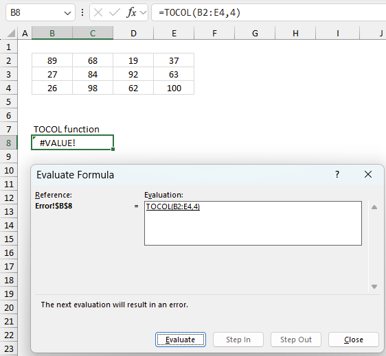
To understand why a formula returns an unexpected value we need to examine the calculations steps in detail. Luckily, Excel has a tool that is really handy in these situations. Here is how to troubleshoot a formula:
- Select the cell containing the formula you want to examine in detail.
- Go to tab “Formulas” on the ribbon.
- Press with left mouse button on "Evaluate Formula" button. A dialog box appears.
The formula appears in a white field inside the dialog box. Underlined expressions are calculations being processed in the next step. The italicized expression is the most recent result. The buttons at the bottom of the dialog box allows you to evaluate the formula in smaller calculations which you control. - Press with left mouse button on the "Evaluate" button located at the bottom of the dialog box to process the underlined expression.
- Repeat pressing the "Evaluate" button until you have seen all calculations step by step. This allows you to examine the formula in greater detail and hopefully find the culprit.
- Press "Close" button to dismiss the dialog box.
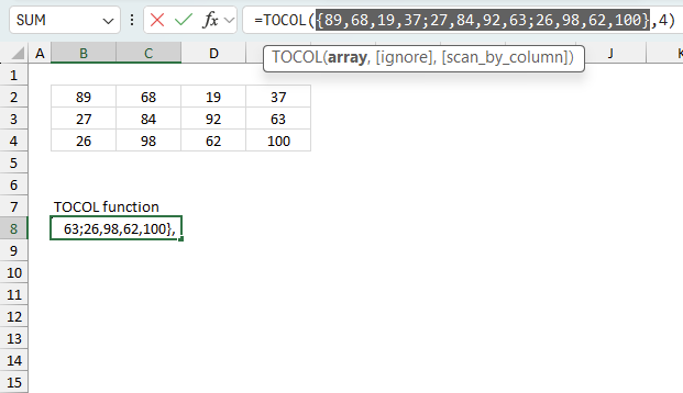
There is also another way to debug formulas using the function key F9. F9 is especially useful if you have a feeling that a specific part of the formula is the issue, this makes it faster than the "Evaluate Formula" tool since you don't need to go through all calculations to find the issue.
- Enter Edit mode: Double-press with left mouse button on the cell or press F2 to enter Edit mode for the formula.
- Select part of the formula: Highlight the specific part of the formula you want to evaluate. You can select and evaluate any part of the formula that could work as a standalone formula.
- Press F9: This will calculate and display the result of just that selected portion.
- Evaluate step-by-step: You can select and evaluate different parts of the formula to see intermediate results.
- Check for errors: This allows you to pinpoint which part of a complex formula may be causing an error.
The image above shows cell reference B2:E4 converted to hard-coded value using the F9 key.
Tips!
- View actual values: Selecting a cell reference and pressing F9 will show the actual values in those cells.
- Exit safely: Press Esc to exit Edit mode without changing the formula. Don't press Enter, as that would replace the formula part with the calculated value.
- Full recalculation: Pressing F9 outside of Edit mode will recalculate all formulas in the workbook.
Remember to be careful not to accidentally overwrite parts of your formula when using F9. Always exit with Esc rather than Enter to preserve the original formula. However, if you make a mistake overwriting the formula it is not the end of the world. You can “undo” the action by pressing keyboard shortcut keys CTRL + z or pressing the “Undo” button
10.3 Other errors
Floating-point arithmetic may give inaccurate results in Excel - Article
Floating-point errors are usually very small, often beyond the 15th decimal place, and in most cases don't affect calculations significantly.
Useful resources
TOCOL function - Microsoft support
Excel TOCOL function - convert range to single column
'TOCOL' function examples

This post explains how to lookup a value and return multiple values. No array formula required.
This article describes an array formula that compares values from two different columns in two worksheets twice and returns a […]
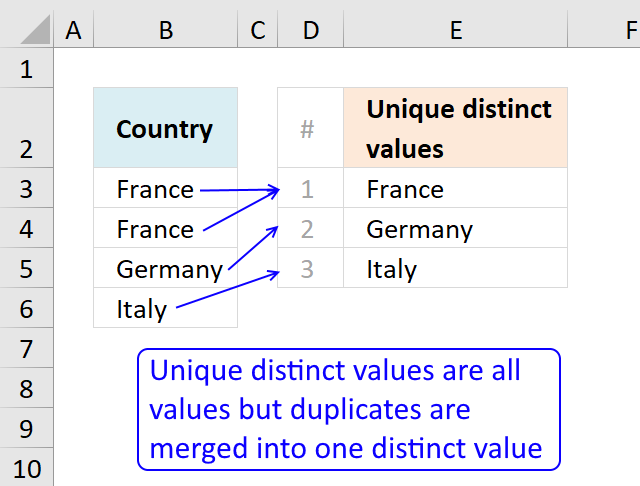
This article describes how to count unique distinct values. What are unique distinct values? They are all values but duplicates are […]
Functions in 'Array manipulation' category
The TOCOL function function is one of 11 functions in the 'Array manipulation' category.
How to comment
How to add a formula to your comment
<code>Insert your formula here.</code>
Convert less than and larger than signs
Use html character entities instead of less than and larger than signs.
< becomes < and > becomes >
How to add VBA code to your comment
[vb 1="vbnet" language=","]
Put your VBA code here.
[/vb]
How to add a picture to your comment:
Upload picture to postimage.org or imgur
Paste image link to your comment.
Contact Oscar
You can contact me through this contact form