Merge cell ranges into one list
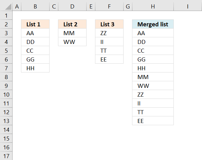
The above image demonstrates a formula that adds values in three different columns into one column.
Table of Contents
- Merge three columns into one list - Excel 365
- Merge three columns into one list - earlier Excel versions
- Merge three columns into one list - Excel 2003 and earlier versions
- Get Excel file
- Combine cell ranges ignore blank cells - UDF
- Merge, sort and remove blanks from multiple cell ranges - UDF
- Consolidate sheets - VBA
- Merge two columns - Excel 365
- Merge two columns - earlier Excel versions
1. Merge three columns into one list - Excel 365
Excel 365 subscribers can access new array manipulation formulas that make working with arrays and cell ranges much easier, one of those new functions is the VSTACK function.
It allows you to merge multiple cell ranges vertically, meaning the second cell range/array is joined below the first cell range/array. The result is a dynamic array formula that spills values below as far as needed.
This example shows how to merge three nonadjacent cell ranges with different sizes, cell range B3:B7 has five values. Cell range D3:D4 has two values, and F3:F6 has four values. The formula is entered in cell H3 and the array values are spilled to cell H3 and cells below as far as needed.
Excel 365 dynamic array formula in cell H3:
Explaining formula
The VSTACK function combines cell ranges or arrays. Joins data to the first blank cell at the bottom of a cell range or array (vertical stacking)
Function syntax: VSTACK(array1,[array2],...)
2. Merge three columns into one list - earlier Excel versions
This example works in earlier Excel versions from 2007 to Excel 2019, it requires a more complicated formula because these versions don't have the VSTACK function.
The IFERROR function is used a lot in this example and I want to warn you that it also handles all formula errors, this may
Formula in H3:
Copy cell H2 and paste to the cells below.
Explaining formula in cell H2
The IFERROR function moves the calculation to the next part (formula2) when the first part (formula1) begins to return errors. That is also true for the second part (formula2), when errors occur the calculation continues with the third part (formula3)
IFERROR(IFERROR(formula1, formula2), formula3)
Formula1 extracts values from List1. Formula2 extracts values from List2. Formula3 extracts values from List3.
Step 1 - Count cells vertically
The ROWS function counts rows in a cell reference. H2:$H$2 is special, it expands as the formula is copied to the cells below.
ROWS(H2:$H$2) returns 1.
Step 2 - Return value
The INDEX function returns values from a cell range based on a row number and column number.
INDEX($B$3:$B$7, ROWS(H2:$H$2)) returns "AA" in cell H3.
Step 3 - Loop
When the formula starts returning errors the second part of the formula begins.
INDEX($D$3:$D$4, ROWS(H2:$H$2)-ROWS($B$3:$B$7))
It also takes into account the number of values returned from the first cell range, for example in cell H8:
INDEX($D$3:$D$4, ROWS(H7:$H$2)-ROWS($B$3:$B$7)) returns "MM" in cell H8.
3. Merge three columns into one list - Excel 2003 and earlier versions
Formula in cell H3:
Named ranges
List1 (A2:A6)
List2 (B2:B3)
List3 (C2:C5)
4. Get Excel file
merge-three-columns_excel_2003.xls
5. Combine cell ranges ignore blank cells - UDF
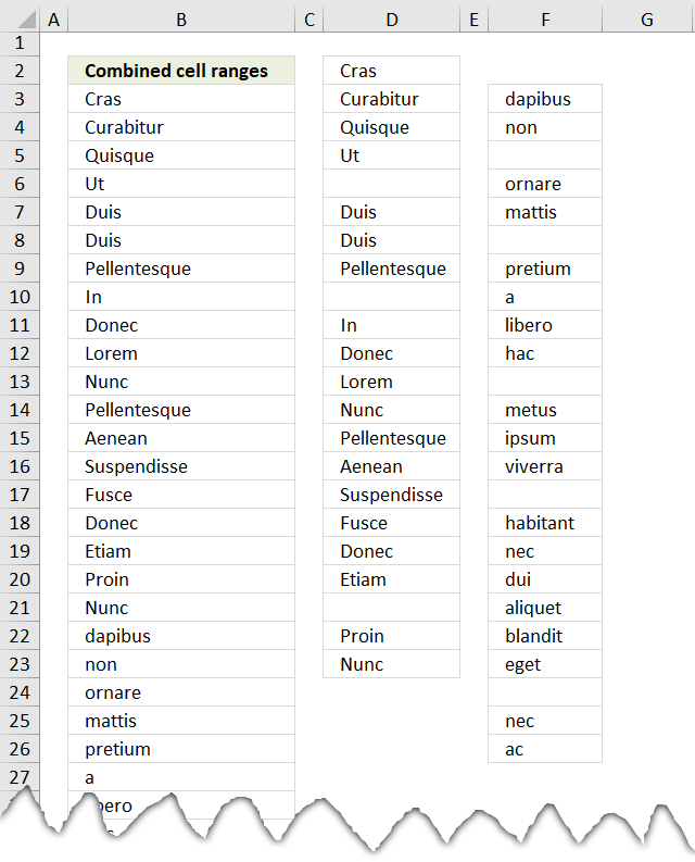
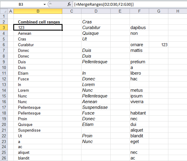
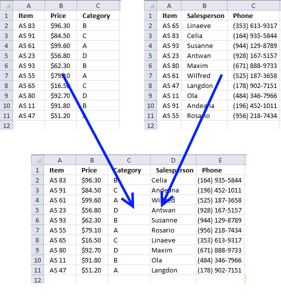
The image above demonstrates a user defined function that merges up to 255 cell ranges and removes blanks. I will also show you how to sort these values.
A user defined function is a custom function in Excel than anyone can build, you simply copy the code below to a module in the Visual Basic Editor and then enter the function name and arguments in a cell.
I have articles that shows you how to combine two and three columns using array formulas. Check out this article that demonstrates how to Merge tables based on a condition.
Array formula in cell range B3:B70:
5.1 How to create an array formula
- Select cell range B3:B70.
- Copy (Ctrl + c) above array formula.
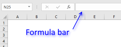
- Paste (Ctrl + v) array formula to formula bar.
- Press and hold Ctrl + Shift.
- Press Enter once.
- Release all keys.
5.2 VBA code
'Name function and declare arguments
Function MergeRanges(ParamArray arguments() As Variant) As Variant()
'Declare variables and data types
Dim cell As Range, temp() As Variant, argument As Variant
Dim iRows As Integer, i As Integer
'Redimension temp in order to let it grow if needed
ReDim temp(0)
'Iterate through each cell range
For Each argument In arguments
  'Iterate through each cell in cell range
  For Each cell In argument
    'If cell not equal to nothing
    If cell <> "" Then
      'Save cell value to array variable
      temp(UBound(temp)) = cell
      'Add another container to array
      ReDim Preserve temp(UBound(temp) + 1)
    End If
  Next cell
Next argument
'Remove container from array
ReDim Preserve temp(UBound(temp) - 1)
'Count cells occupied by user defined function
iRows = Range(Application.Caller.Address).Rows.Count
'Add containers
For i = UBound(temp) To iRows
  'Add another container
  ReDim Preserve temp(UBound(temp) + 1)
  'Save "" to array
  temp(UBound(temp)) = ""
Next i
'Return array
MergeRanges = Application.Transpose(temp)

End Function
5.3 How to add the user defined function to your workbook
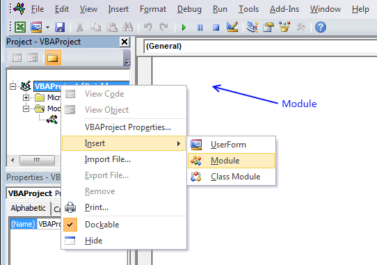
- Press Alt-F11 to open visual basic editor
- Press with left mouse button on Module on the Insert menu
- Copy and paste vba code
- Exit visual basic editor
Sort text from multiple cell ranges combined (user defined function):
Recommended articles
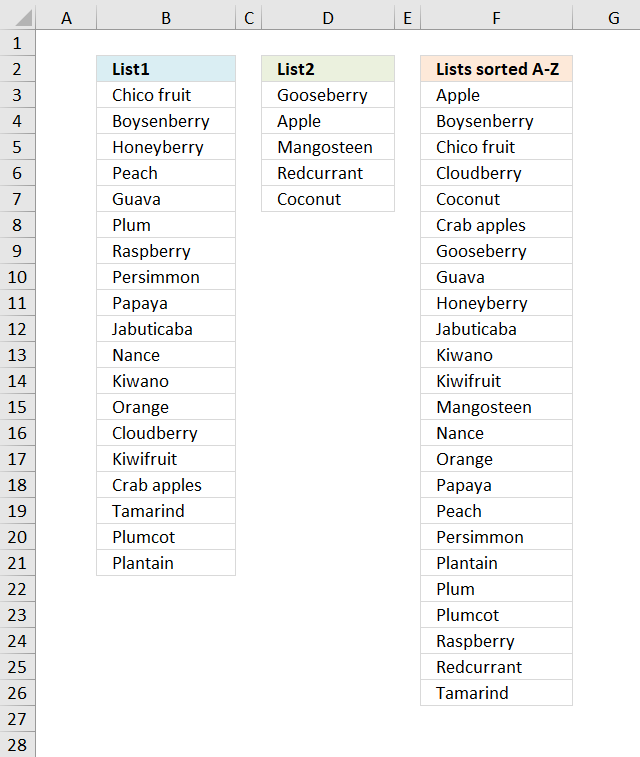
Table of Contents Sort text from two columns combined (array formula) Sort text from multiple cell ranges combined (user defined […]
6. Merge,sort and remove blanks from multiple cell ranges - UDF
I used the "Sort array" function found here: Using a Visual Basic Macro to Sort Arrays in Microsoft Excel (microsoft) with some small modifications.
Function SelectionSort(TempArray As Variant)
    Dim MaxVal As Variant
    Dim MaxIndex As Integer
    Dim i As Integer, j As Integer

    ' Step through the elements in the array starting with the
    ' last element in the array.
    For i = UBound(TempArray) To 0 Step -1

        ' Set MaxVal to the element in the array and save the
        ' index of this element as MaxIndex.
        MaxVal = TempArray(i)
        MaxIndex = i

        ' Loop through the remaining elements to see if any is
        ' larger than MaxVal. If it is then set this element
        ' to be the new MaxVal.
        For j = 0 To i
            If TempArray(j) > MaxVal Then
                MaxVal = TempArray(j)
                MaxIndex = j
            End If
        Next j

        ' If the index of the largest element is not i, then
        ' exchange this element with element i.
        If MaxIndex < i Then
            TempArray(MaxIndex) = TempArray(i)
            TempArray(i) = MaxVal
        End If
    Next i

End Function
7. Consolidate sheets - VBA

Question:
I have multiple worksheets in a workbook. Each worksheets is project specific. Each worksheet contains almost identical format. The columns I am interested in each worksheets are "Date Plan", "Date Completed" and "variance" and "Project Code"I then want data from all these column to be extracted in a Report worksheet and later want to do a trend chart by sorting all dates in chronological order.
Key bit to start is how do I get data out from worksheets. Essentially I want all the data without any loss. There are chances that some of the data between worksheet1 & 2 could be identical, apart from project code.
Also, preference is that this coding or formula should work for any future addition to worksheet data and workbook worksheets.
Answer:
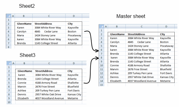
This VBA code copies all values from each column header in each sheet to "consolidate" sheet. You can choose which sheets to consolidate, cell A2 and down. See picture above.
You can also choose what column headers to consolidate. Cell B1 and cells to the right. Remember column headers must be on row 1 in each sheet. Cell values don't have to be contiguous in each sheet.
VBA
Sub Consolidate()
Application.ScreenUpdating = False
'Dim
Dim csShts        As Range
Dim clmnheader        As Range
Dim sht As Worksheet
Dim LastRow As Integer
Dim i As Long
Set csShts = Worksheets("Consolidate").Range("A2")
Set clmnheader = Worksheets("Consolidate").Range("B1")
'Iterate sheet cells on sheet "consolidate"
Do While csShts <> ""
    ' Iterate all sheets to find a match between sht and csShts
    For Each sht In Worksheets
    'Find a matching sheet
    i = 0
    If sht.Name = csShts Then
        'Select sheet
        sht.Select
        'Select cell A1 on sheet
        Range("A1").Select
        'Iterate columnheaders on sheet
        Do While Selection <> ""
            'Iterate column headers on consolidate sheet
            Set clmnheader = Worksheets("Consolidate").Range("B1")
            Do While clmnheader <> ""
                'Find matching column headers on consolidate sheet
                 against column headers on current sheet
                If clmnheader.Value = Selection.Value Then
                    'Find last row in column
                    LastRow = ActiveSheet.Cells.Find(What:="*", _
                    SearchDirection:=xlPrevious, _
                    SearchOrder:=xlByRows).Row
                End If
                    'Save maximum last row number on current sheet
                    If LastRow > i Then
                        i = LastRow
                    End If
                'Move to next column header on consolidate sheet
                Set clmnheader = clmnheader.Offset(0, 1)
            Loop
        ActiveCell.Offset(0, 1).Select
        Loop
        sht.Select
        Range("A1").Select
        Set clmnheader = Worksheets("Consolidate").Range("B1")
        'Iterate columnheaders from beginning on current sheet
        Do While Selection <> ""
            Set clmnheader = Worksheets("Consolidate").Range("B1")
            'Iterate column headers on consolidate sheet
            Do While clmnheader <> ""
                If clmnheader.Value = Selection.Value Then
                    Set clmnheader = clmnheader.Offset(1, 0)
                    'Copy range
                    Do While Selection.Row <= i
                        ActiveCell.Offset(1, 0).Select
                       Selection.Copy
                        clmnheader.Insert Shift:=xlDown
                    Loop
                    ActiveCell.Offset(-i, 0).Select
                    Set clmnheader = clmnheader.Offset(-i, 0)
                    'Set clmnheader = clmnheader.End(xlUp)
                End If
                'Move to next column header on consolidate sheet
                Set clmnheader = clmnheader.Offset(0, 1)
            Loop
        'Move to next cell on current sheet
        ActiveCell.Offset(0, 1).Select
        Loop
    End If
    Next sht
'Move to next cell
Set csShts = csShts.Offset(1, 0)
Loop
Sheets("Consolidate").Select
End Sub
Now you can easily sort dates in chronological order and create a trend chart.
Get excel file
(Excel 97-2003 Workbook *.xls)
Remember to backup your original excel file. You can´t undo a macro.
8. Merge two columns - Excel 365
The new VSTACK function, available for Excel 365 subscribers, handles this task easily. In fact, it is built solely to combine cell ranges or arrays.
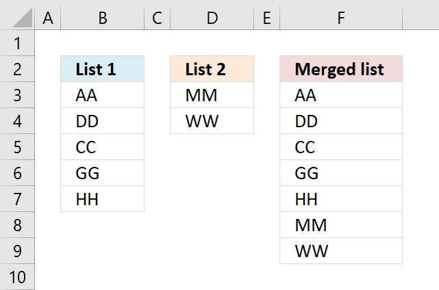
This example shows how to merge two nonadjacent cell ranges with different sizes located in B3:B7 and D3:D5, the result is returned to cell F3 and cells below as far as needed.
This is a new behavior to dynamic array formulas in Excel 365, called spilling meaning values from a dynamic array formula are all returned if adjacent cells are empty.
Excel 365 dynamic array formula in cell F3:
Explaining formula
Step 1 - Populate arguments
The VSTACK function combines cell ranges or arrays. Joins data to the first blank cell at the bottom of a cell range or array (vertical stacking)
Function syntax: VSTACK(array1,[array2],...)
VSTACK(array1,[array2],...) becomes VSTACK(B3:B7, D3:D4)
Step 2 - Evaluate VSTACK function
VSTACK(B3:B7, D3:D4) returns {"AA"; "DD"; "CC"; "GG"; "HH"; "MM"; "WW"}.
9. Merge two columns - earlier Excel versions
This example demonstrates a formula that only works in Excel 2007 and later versions, it utilizes the IFERROR function to move between cell ranges. However, the IFERROR function handles all formula errors and this may make it hard for you to spot other formula errors.
If you are looking for a formula to merge columns based on a condition read this article: Merge tables based on a condition
Formula in F3:
Copy cell C2 and paste it down as far as needed.
Earlier versions of excel, formula in C2:
Copy cell C2 and paste it down as far as needed.
How the formula in F3 works
Step 1 - Extracting List 1
=IFERROR(INDEX($A$2:$A$6, ROWS(C1:$C$1)), IFERROR(INDEX($B$2:$B$3, ROWS(C1:$C$1)-ROWS($A$2:$A$6)), ""))
The ROWS function calculate the number of rows in a cell range.
Function syntax: ROWS(array)
In cell C2: INDEX($A$2:$A$6, ROWS(C1:$C$1)) returns "AA"
In cell C3: INDEX($A$2:$A$6, ROWS(C1:$C$1)) returns "DD"
and so on...
Step 2 - Error when all values in List 1 are processed
IFERROR(INDEX($A$2:$A$6, ROWS(C1:$C$1)), IFERROR(INDEX($B$2:$B$3, ROWS(C1:$C$1)-ROWS($A$2:$A$6)), ""))
In cell C7 something unexpected happens:
In cell C7: INDEX($A$2:$A$6, ROWS(C1:$C$1)) returns "#REF!" error
There are no more values in List 1 so we need to continue on List 2.
IFERROR() takes care of this:
The IFERROR function if the value argument returns an error, the value_if_error argument is used. If the value argument does NOT return an error, the IFERROR function returns the value argument.
Function syntax: IFERROR(value, value_if_error)
Step 3 - Continue with List 2
In cell C7:
=IFERROR(INDEX($A$2:$A$6, ROWS(C6:$C$1)), IFERROR(INDEX($B$2:$B$3, ROWS(C6:$C$1)-ROWS($A$2:$A$6)), "")) returns "MM" in List 2.
Step 4 - Error when all values in List 2 and List 1 are evaluated
In cell C9:
=IFERROR(INDEX($A$2:$A$6, ROWS(C8:$C$1)), IFERROR(INDEX($B$2:$B$3, ROWS(C8:$C$1)-ROWS($A$2:$A$6)), ""))
returns "" (nothing)
Get Excel *.xlsx file
Useful links
Combine data from multiple sheets - Microsoft
Consolidate data in Excel and merge multiple sheets into one worksheet
Consolidate Data From Multiple Worksheets in a Single Worksheet in Excel
Combine merge category
This article demonstrates two formulas, they both accomplish the same thing. The Excel 365 formula is much smaller and is […]
Merge Ranges is an add-in for Excel that lets you easily merge multiple ranges into one master sheet. The Master […]
This article demonstrates techniques on how to merge or combine two data sets using a condition. The top left data […]
Excel categories
102 Responses to “Merge cell ranges into one list”
Leave a Reply
How to comment
How to add a formula to your comment
<code>Insert your formula here.</code>
Convert less than and larger than signs
Use html character entities instead of less than and larger than signs.
< becomes < and > becomes >
How to add VBA code to your comment
[vb 1="vbnet" language=","]
Put your VBA code here.
[/vb]
How to add a picture to your comment:
Upload picture to postimage.org or imgur
Paste image link to your comment.
This article is terrific. Thanks so much for posting this solution!
I do have one question:
Let's say my "List 1" is auto updated and the number of entries in this list will fluctuate. Since the number of entries fluctuates, I would like to select a larger range than I actually have data in currently. The issue is when I make my "List 1" larger than the number of entries, the rows that don't currently have data in them, show up on my combined list as zeros.
So my question is, is there a way to adjust the formula so that when it looks at "List 1" for example, it skips over blank cells and continues to combine the list with "List 2".
Dan,
See this post: https://www.get-digital-help.com/2010/05/18/merge-two-columns-with-possible-blank-cells-in-excel-formula/
I have down loaded the consolidated file and it does not appear to work the way I expected.
I am looking to combine cashflow worksheets for multiple projects. The row headings are the same for each project but the column heading varies (they are set as end of month dates)
The issue with normal consolidation is that each sheet has to be identical. But because each project starts and stops at different months the consolidation is messy
Can I use your example and modify it.
You can use it and modify it.
It is an interesting question and I´ll post an answer as soon as possible.
the code has it that all the headers must be in row 1 of each sheet. How would you modify if the headers all on the 13th row on each sheet?
Neville Ash,
Read https://www.get-digital-help.com/2010/09/06/consolidate-sheets-in-excel-part-2/
Have I missed something? I found the formula listed above worked just as well *without* entering it as an array formula.
Excel solution either way.
typo... *excellent solution either way
Thanks!!
Thanks A LOT!!! I really mean it. Lifesavers you guys are!
Can you translate this into an earlier version of Excel please....I REALLY wish I had a clue how to use VBA (or how to write these formulas myself!)
Shawna,
Yes, the formula is large but it is not an array formula. I have included the excel 2003 solution in this blog post. Read above and you can also get an Excel 2003 file.
Thanks, now we're cooking!! Anyway to remove the blanks from the resulting "merged" list?
nevermind...sorry I bothered you, I can't get the new formula to work at all, so it's pointless. Thanks for the time and effort anyway.
Hmmm, tried again and I got it to work, but I still come up with zeros if one of my Lists has a blank. This is SO frustrating!!
Shawna,
I hope this user defined function works in excel 2003:
Function MergeRanges(ParamArray arguments() As Variant) As Variant()
Dim cell As Range, temp() As Variant
ReDim temp(0)

For Each argument In arguments
  For Each cell In argument
    If cell <> "" Then
      temp(UBound(temp)) = cell
      ReDim Preserve temp(UBound(temp) + 1)
    End If
  Next cell
Next argument

ReDim Preserve temp(UBound(temp) - 1)
MergeRanges = Application.Transpose(temp)

End Function
Where to copy the code?
Press Alt-F11 to open visual basic editor
Press with left mouse button on Module on the Insert menu
Copy and paste the user defined function into module
Exit visual basic editor
How to use user defined function in excel
Select a cell
Type MergeRanges(A1:C10, Sheet2!A3:B10) in formula bar, you can have as many range arguments you like.
Press Ctrl + SHIFT + ENTER
Add more cells to your selection.
Press with left mouse button in Formula bar.
Press Ctrl + SHIFT + ENTER
I wish I could try it, but I don't know how to create VBA. I'm a novice, though I did try a few times from random directions online, but it didn't work. :(
LOL, sorry...you gave me directions to follow, DUH! It's early, I'm not awake yet, so the attention hasn't kicked in. I'll let you know how I make out when I get to work. Thanks!
Nope...I set up the following example:
Heading1 Heading2 Heading3 Merge aa aa bb hh bb
cc ii 1 cc
2 dd
dd jj 3 dd
ee ee
kk 4 ff
ff ff
gg gg
#VALUE!
#VALUE!
#VALUE!
I pasted the code in the VBA module and typed the statement:
=MergeRanges(A2:A11, B2:B11, C2:C11) into the Merge cell. Then copied it down. However, notice only the A range merged. Also, the merged column repeated dd and ff (the only ones preceeded by a space). Any idea what I messed up?
Shawna,
Get the Excel file
udf-merge-ranges.xls
Udf is in cell range B3:B24, sheet1.
Can we please discuss via email so I can attach an example of what I am doing? My typed example above was obviously worthless! LOL
Thanks! :)
Shawna,
Yes, you can use the contact form on this page: Contact me
Hello,
I gotr your Excel workbook and wanted to know how to combine lists that are 2000 items in length?
Hi,I have little experience with excel.Could someone point out how to run this array formular? I entered the formular into the cell but it didn't give me the list.
Btw,I am using a mac.And the formular doesn't seem to work with openoffice on my linux anyway.
Jane,
It looks like IFERROR function and ISERROR function don´t exist in OpenOffice.
Oscar,
Thanks!If I want to merge multiple,say 5,columns in the same manner,how should I change the parameters then?Thanks and I am using excel now.
Try this udf:Combine cell ranges into a single range while eliminating blanks
is there a way to merge two columns of dates in this similar way but only combine the dates that appear on both columns? ie. without duplicating them in the newly created column?
macutan,
Array formula in cell D3:
Excel file
merge-two-columns-return unique distinct values.xlsx
(Excel 2007 Workbook *.xlsx)
Thank you Oscar for your reply,... I am using Excel 2003, which is probably why I am getting #NAME? in the cells where the merged list is supposed to appear... Any ideas as to how can i get this working in my excel version?
Also please note that as per list1 and list2 shown above, i would be looking for the merged list to have ONLY duplicate dates in it (as in dates that appear in both list1 and list 2) so in this case the merged list would display (also if possible in descending or ascending order) 2011-01-01 as that is the date that is in both lists.
Any guidance will be greatly appreaciated
Rgds
macutan
macutan
Array formula:
Read this post: How to find common values from two lists
Thank you Oscar, I have just tried to run your formula in an array but i am getting 2011-01-01 repeated until the end of the array instead of what you are seeing on the Merged list.
also, do you know how to modify the final array formula so that the dates come out descending.
macutan
Filter common dates from two columns and return unique distinct dates sorted smallest to largest
Array formula in cell D3:
How to create an array formula
Copy (Ctrl + c) and paste (Ctrl + v) array formula into formula bar.
Press and hold Ctrl + Shift.
Press Enter once.
Release all keys.
Get the Excel file
sort-common-dates-from-two-columns.xls
Excel 97-2003 *.xls
Thanks a lot Oscar!!
This is great! Almost exactly what I was looking for.
I got the consolidate sheet and I am able to get all of my data to consolidate fine. If I update something and press consolidate again, it displays a second set of data instead of replacing what showed up the upon the first press with left mouse button. Is there a way to replace the existing data on the consolidate sheet when ever I press with left mouse button on "consolidate"?
also, after the 540th row, only half of the columns show up. any ideas? all told, I have 14 columns and 921 rows.
Stephen,
This line deletes all values in range B2:E65536:
Worksheets("Consolidate").Range("B2:E65536") = ""
Copy and paste after this line:
Dim i As Long
Get the Excel file
stephen.xls
I've never used the INDEX function before and this is a great use for it. My last puzzle is to automate the length of the merge column. Been trying to do with with a dynamic table height but no luck. anyone got ideas?
Cheers
Windfery,
I am not sure I understand, automate the length of the merge column?
You want the named ranges to expand whenever new values are added, right?
Windfery,
I updated this blog post.
hi
i have two sheets in my workbook
sheet1 :
A14:A200 = item code
E14:E200 = quantity
sheet2 :
column "C" = item code
column "I" = Quantity
i want if
sheet1 :
A14=101, A15=102 & E14=4&E15=5
sheet 2 :
C15=101, c22=102 & C15=20, C22=25
then,,,
vba search for 101 nd 102 in sheet 2, column c
and add quantity
ans could be
C15=24 & E15=30
can any1 help me for this
Deepak,
Can you provide som sample data?
Hey Oscar!!
Many thanks for sharing your excel knowledge...Ive been trying to figure this out for a while!...
I copied the formula into my worksheet (Im using excel 2003), but (and I cant see why), but the formula has only copied the first named range column (GN_LIST in column H) into the merged column (column M).
If I change the very last range name to the second list name (SH_LIST in column L), then the second column only is entered into the merged column.
My formula is as follows:
=IF(ISERROR(INDEX(GN_LIST, ROWS($M$1:M2))), IF(ISERROR(INDEX(SH_LIST, ROWS($M$1:M2)-ROWS(GN_LIST))), "", INDEX(SH_LIST, ROWS($M$1:M2)-ROWS(GN_LIST))), INDEX(GN_LIST, ROWS($M$1:M2)))
Can you PLEASE help?!? I am baffled...
Regards
I have resolved this now! Originally I wanted to define two separate columns as the two ranges as the data being impoted into them varies month by month i.e the data is dynamic. Through experimentation and testing, I discovered that your formula only works for statically defined ranges. It would be great to be able to adapt your formula to be used with dynamic ranges, but that is, sadly, beyond my excel scope and knowledge. If you are able to provide this, I would be deeply grateful, but if you are not, then I will use my work-around. Many thanks.
Dan,
Get the Excel 2003 *.xls file
merge-two-columns-dynamic-ranges1.xls
Received with many thanks!!!
I noticed that you have limited the height definition for the range to 10,000 cells. Is there any particular reason for this (ie. slower processing when more cells are included in the range), or can the height theoretically be increased down to cell 65,536?
Dan,
There is no partcular reason, it can be increased down to cell 65,536.
Thanks for commenting!
here is a version i used that auto counts the columns so you don't have to have your "list1" range = the range. I used this to combine multiple columns. Please mind that i didn't name my first indexranges which wouuld have simplified alot
=IFERROR(INDEX($AL$2:$AL$26, ROWS(BW$1:$BW15)), IFERROR(INDEX($AU$2:$AU$26, ROWS(BW$1:$BW15)-COUNT($AL$2:$AL$26)), IFERROR(INDEX($BA$2:$BA$26, ROWS(BW$1:$BW15)-SUM(COUNT($AL$2:$AL$26), COUNT($AU$2:$AU$26))), IFERROR(INDEX($BH$2:$BH$26, ROWS(BW$1:$BW15)-SUM(COUNT($AL$2:$AL$26), COUNT($AU$2:$AU$26), COUNT($BA$2:$BA$26))), IFERROR(INDEX($BO$2:$BO$26, ROWS(BW$1:$BW15)-SUM(COUNT($AL$2:$AL$26), COUNT($AU$2:$AU$26), COUNT($BA$2:$BA$26), COUNT($BH$2:$BH$26))), "")))))
Hey Oscar,
i am trying to merge 4 columns into one list but i think i have run into an issue. Can you help? I have already substitued my named ranges. One thing i have to note is that these named ranges are created using the following formula =OFFSET(References!$N$1,1,0,COUNTA(References!$N:$N)-1,1) so that i can use my named ranges in a dropdown box with data validation. These named ranges are always being updated so i dont want to have to continually change the range of the named reference. Let me know if you can help.
thanks JOEY
=IFERROR(INDEX(Phatec_Local_DIDs, ROWS(AM2:$AM$2)), IFERROR(INDEX(Phatec_Toll_Frees, ROWS(AM2:$AM$2)-ROWS(Phatec_Local_DIDs)), IFERROR(INDEX(Comcast_Local, ROWS(AM2:$AM$2)-ROWS(Phatec_Local_DIDs)-ROWS(Phatec_Toll_Frees)), IFERROR(INDEX(Comcast_Toll_Free, ROWS(AM2:$AM$2)-ROWS(Phatec_Local_DIDs)-ROWS(Phatec_Toll_Frees)-ROWS(ComCast_Local)),"")))) + CTRL + SHIFT + ENTER
one other thing that maybe you can help me with? i was able to use your two column method for combining two named ranges. Works great. The only issue now is when i go to sort the list it only sorts list one then sorts list two in the same column. Not sure if i explained that right but below is what i am experiencing.
List one:
216
220
221
223
305
311
314
315
360
361
501
505
511
List two
200
202
244
250
320
350
399
400
400
401
402
403
449
499
514
550
557
590
598
599
600
601
607
666
After using the sort feature it shows like this? each of the cells are in a table. Its like it sorts list one first then after sorting list one it sorts list two?
216
220
221
223
305
311
314
315
360
361
501
505
511
200
202
244
250
320
350
399
400
400
401
402
403
449
499
514
550
557
590
598
599
600
601
607
666
Joey,
Question 1:
You can see the logic behind this formula:
Merge three columns into one list in excel
and then adapt it to your formula.
Joey,
Question 2:
I recommend converting the formulas to values before sorting.
1. Select range
2. Copy (Ctrl + c)
3. Press with right mouse button on the same range.
4. Press with left mouse button on "Paste Special.."
5. Press with left mouse button on "Values"
6. Press with left mouse button on OK
This article is great.
Exactly what I needed.
Thanks so much for posting.
;-)
Thanks for commenting!
Hi Oscar,
Here I found one interesting solution to merge table to single row. It could be useful for you :)
https://www.cpearson.com/excel/TableToColumn.aspx
I modified formula with INDEX() function (array formula) and like result :)
=INDEX(Table;1+MOD(ROW()-ROW(MergedRange);ROWS(Table));1+TRUNC((ROW()-ROW(MergedRange))/ROWS(Table);0))
Best regards
The solution is to merge table to single column, not row...
BatTodor,
Thanks for sharing!
Great article. I have to combine 200 columns into one list. I know. I tried steps from 'Combine cell ranges into a single range while eliminating blanks' UDF, but looks like typing the formula itself is going to be a big deal. Any advice? (To give a bit of a background, I am trying to compare 200 columns to one column of data and figured it would be easier if I combine all 200 into one column and then compare, it would be easy).
Jinesh,
You want to know how to simplify/automate typing 200 column ranges in a udf?
Good question! I don´t know but I believe a macro should be able to return addresses of cell ranges populated with values.
Read this post:
Extract cell references from all cell ranges populated with values in a sheet
Redim Preserve does not execute all that quickly, so it is usually a good idea to avoid using it too often. Here is an alternate function to the one you posted which avoids them altogether...
Function MergeRanges(ParamArray Arguments() As Variant) As Variant() Dim X As Long, Index As Long, Cell As Variant, TempArray As Variant, Done As Boolean ReDim TempArray(1 To Application.Caller.Count) Index = 1 For X = LBound(Arguments) To UBound(Arguments) For Each Cell In Arguments(X) If Len(Cell.Value) Then TempArray(Index) = Cell.Value Index = Index + 1 If Index > UBound(TempArray) - LBound(TempArray) + 1 Then Done = True Exit For End If End If Next If Done Then Exit For Next For X = Index To UBound(TempArray) TempArray(X) = "" Next MergeRanges = Application.Transpose(TempArray) End FunctionRick Rothstein (MVP - Excel),
I didn´t know! I am curious, I have to do some speed tests.
Thank you for your valuable contribution!
This works well, but doesn't work if you have strings over 255 letters long! Any idea how to work around that? Thanks, Tom
Hello Oscar,
thanks for updating this code...
can you do a favour,,,, if i am using this code to consolidate the data,it is working fine for me but can i get the sheet(project) name as well against the data, so that i can track, from which project i pick the number,
[...] [...]
I’m building an S-Curve Chart from disaster Condition Excel Spread sheet, that should reflect in the end: Plan and forecast weekly bars info and plan and forecast cumulative progress curves.
Take Plan Date Column & Using Pivot Table Fields: Row Labels and Values (count) I get an output such as:
Columns: a – Plan Date, b – linked value
Repeat above for Forecast Date using same Pivot Table Fields:
Columns: c – Forecast Date, d – linked value
Now I have 4 Columns: (a) Date + (b) linked value / (c) Date + (d) linked value.
Challenge, as I see it:
Compare dates columns a and c, c and a, find unique dates, somehow combine them into one column, but somehow keep linked value associates with each date:
So in the end I would get:
Column A – Date (for both Plan and Forecast)
Column B – Linked to Plan Date Value (if date is related to forecast value, then put 0 in plan column B for this row)
Column C – Linked to Forecast Date Value (if date is related to Plan value, then put 0 in forecast column C for this row)
So Ultimate goal is to have this database ready for a chart.
I’m sure there are various ways of manually doing it, but I also predict there must be a way of doing it all through Macro.
I have zero marco experience, so came to this forum with desperate need for a help. Please.
Oscar
thank you so much, it is just wonderful tricks you show here, now i can get rid of that macro in my excel dashboard.
thank you again and happy new year
Brilliant work, I converted List1, List2,List3 into dynamic range.
ALIST = =OFFSET($A$1,0,0,COUNTA($A:$A),1)
BLIST = =OFFSET($B$1,0,0,COUNTA($B:$B),1)
CLIST = =OFFSET($C$1,0,0,COUNTA($C:$C),1)
DLIST = =OFFSET($D$1,0,0,COUNTA($D:$D),1)
Here link to solution with screenshot.
https://stackoverflow.com/questions/14774806/how-to-combine-4-column-into-1-column
Zuberr,
thank you!
[...] all, Please first have a look at this link so that you may follow me: Merge two columns into one list in excel | Get Digital Help - Microsoft Excel resource I would like to combine List1 and List2 into a 3rd named range called List3. I was wondering if [...]
Hi Oscar
Hope you are well!...
I have not asked for your assistance since January of last year because, after your invaluable help, I was able to complete the task I was working on.
I am now re-visiting the work as amendments need to be made and I find myself stuck again, as I have not Excel so indepth since.
Maybe you can help...
I asked you about merging to columns of dynamic data with possible blanks into one sorted column and you were able to help me do this.
An example of one such equation is provided below (I'm using 2003):
=IF(ISERROR(INDEX(ListGN, ROWS($O$1:O2))), IF(ISERROR(INDEX(ListSH, ROWS($O$1:O2)-ROWS(ListGN))), "", INDEX(ListSH, ROWS($O$1:O2)-ROWS(ListGN))), INDEX(ListGN, ROWS($O$1:O2)))
I now need to add a third column to this equation, and although I have a rough idea of what to do, I was hoping you could help me out as I'm rusty.
Many thanks!!
Dan,
Merge three columns into one list
Hi Oscar!
Many thanks for getting back to me. I had already seen this page but its not giving me what I want in the way as the previous expression posted above.
I have definied the third dynamic range, ListARGN
=OFFSET(core_calculations!$N$2,0,0,COUNTA(core_calculations!$N$2:$N$65536),1)
but am finding it quite difficult to logically workout how to expand the existing equation to take into account the new column of numbers.
I suppose an alternatiove would be to add another column to then merge and sort the first merged/sorted column with the new column. It should produce the same result but is not as tidy...
Can you assist at all? It would be a massive help!
Regards
Hi Oscar again!
I have just worked out what I was doing before and must admit that I got myself into a pickle! (I said I was rusty - haha)!
So, I have taken another look at your merge three columns into one list example and got things working correctly!
So, I must thank you again for this amazing website and your wonderful assistance!
Kindest regardss
Dan, can you explain your logic for the additional column? I have a total of 5 columns I need to convert into one list. Each column increases by time so they have to be individual columns. I am able to get the 3 columns to merge into one. Thank you very much!!!!!!!!!!!!!!!!!
Hi Oscar,
This is a great thread! I am having some trouble. I want to combine 2 lists into one list. I want only one record of duplicates and I want the unique items from both lists to be returned as well. The formula above is only returning me the first value from List 1 all the way down the column.
Thanks!
Jamie
Jamie,
The formula above is only returning me the first value from List 1 all the way down the column.
Make sure you entered the formula as an array formula. Also check your cell references, they might be wrong.
This code does exactly what I was looking for, except in one case: if the fields being consolidated have formulas that refer to columns I'm not consolidating (ie it returns #ref or #value errors). Is there any way to amend the code to "paste values"?
I've combined several cell ranges across several sheets, how would I eliminate the duplicate cells using the vba provided?
Trying to generate a list based on several cell ranges on Sector A-P sheets and combine totals on a Totals sheet.
Using formula above to combine 2 data tables on separate sheets into a new sheet in one work book. I made sure the formula is correct and entered as array.
{=IFERROR(INDEX(Table_Query_from_QuickBooks_Data[[#Headers],[Name]], ROWS(A1:$A$1)), IFERROR(INDEX(Table_Query_from_QuickBooks_Data9[Name], ROWS(A1:$A$1)-ROWS(Table_Query_from_QuickBooks_Data[[#Headers],[Name]])), ""))}
It is only returning the data from table 1.
Does it have to be one table?
This is a very useful formula. But, here the list names have fixed ranges and if the ranges expand or reduces, then the formula does not hold good. For example, list1 range A1:A20 with data upto A7, list2 range B1:B20 with data upto row b17 and list3 range C1:C20 with data upto C10. In simple words, the ranges need to be dynamic. Can anybody help with a formula (not Vba). Regards.
R Vijayakumar,
Try this:
https://www.get-digital-help.com/2011/05/17/excel-charts-use-dynamic-ranges-to-add-new-values-to-both-chart-and-drop-down-list/
i have tried in different ways and found this array formula works....
=IFERROR(IFERROR(IFERROR(INDEX(MultiPlyYarnPRCount, MATCH(0, COUNTIF(L$7:$L7, MultiPlyYarnPRCount), 0)), INDEX(MultiPlyYarnDHPRCount, MATCH(0, COUNTIF(L$7:$L7, MultiPlyYarnDHPRCount), 0))),INDEX(MultiPlyYarnDHCRCount, MATCH(0, COUNTIF(L$7:$L7, MultiPlyYarnDHCRCount),0))),"")
MultiPlyYarnPRCount (I8:I100),MultiPlyYarnDHPRCount (J8:J100) and MultiPlyYarnDHCRCount (K8:K100) are three ranges in three columns, each having varying lengths of data i.e. first range has data in only one row, second range 23 rows and third one has 18 rows of data. This formula works fine.
I request your suggestion for fine-tuning the formula if possible.
Regards,
I really need help!
Have similar but bigger issue
Have three columns in excel:
Column A: Category
Column B: Value
Column C: Value
I want to consolidate the list such that if I have a row like:
A1=Car | B1=Ford | C1=Toyota
A2=Scooter | B1=Honda | C1=(blank)
Gives me a result:
A1=Car | B1=Ford
A2=Car | B2=Toyota
A3=Scooter | A3=Honda
Sorry, correction:
I want to consolidate the list such that if I have a row like:
A1=Car | B1=Ford | C1=Toyota
A2=Scooter | B2=Honda | C2=(blank)
Gives me a result:
A1=Car | B1=Ford
A2=Car | B2=Toyota
A3=Scooter | B3=Honda
How can I merge 5 columns?
thanks
anthony,
The easiest way to go is to use a simple user defined function:
Function MergeRanges(ParamArray arguments() As Variant) As Variant()
Dim cell As Range, All As String
For Each argument In arguments
  For Each cell In argument
    All = All & cell & ","
  Next cell
Next argument
MergeRanges = Application.Transpose(Split(All, ","))
End Function
Where to copy the code?
Press Alt-F11 to open visual basic editor
Press with left mouse button on Module on the Insert menu
Copy and paste the user defined function into module
Exit visual basic editor
How to use user defined function in excel
Select a cell
Type =MergeRanges(A1:C10, Sheet2!A3:B10) in formula bar, you can have as many range arguments you like.
Press Ctrl + SHIFT + ENTER
Add more cells to your selection.
Press with left mouse button in Formula bar.
Press Ctrl + SHIFT + ENTER
Oscar, your formula for merging two columns into one, works great! However, I am dealing with dates. I want to sort range to oldest to newest. I tried re-formatting and it seems to not work. Your comments or suggestions would be greatly appreciated. Thank you in advance -Carl
Carl Carter,
I don't know how to do that with a formula or array formula. It is possible with a User Defined Function.
Carl Carter
The UDF found on this webpage lets you merge and sort values from multiple cell ranges:
https://www.get-digital-help.com/sort-text-cells-alphabetically-from-two-columns-using-excel-array-formula/#sortudf
Thanks for your article, it inspired me to come up with the following two formulas. The first combines two columns of numbers into one without having to first define the length of both Array ranges or use the IFERROR. Assuming that the two list of numbers are in columns A and B,
=IF(ROWS($1:1)>COUNT($A:$A,$B:$B),"",IF(ISNUMBER($A2),$A2,INDEX($B:$B,ROW()-COUNT($A:$A))))
The crux of the formula is "IF(ISNUMBER($A2),$A2,INDEX($B:$B,ROW()-COUNT($A:$A))))". The beginning "IF(ROWS($1:1)>COUNT($A:$A,$B:$B)" returns a blank cell if the row number is greater than the combined count of both arrays, so that the formula can be copied down as far as one likes.
A simpler solution, if one wants to have the combined list sorted is the following:
=IF(ROWS($1:1)>COUNT($A:$A,$B:$B),"",SMALL(($A:$A,$B:$B),ROWS($1:1)))
Using nested brackets within the SMALL function, more than one array can be combined together. The added advantage of this formula is that it can handle blank cells or even cells with text within the desired list of numbers. Thanks again, Sam
Sam,
Thank you for your comment.
SAM the ****** genius
Hi people,
Here's a solution i'm trying to solve using the functionality/formula provided at the top of this post .
Let's substitute List1, List 2 and List3 ranges with dynamic ranges that are using offsets when referring to data filter results elsewhere in my workbook. these dynamic ranges sometimes return no data as there are no results at times in my filters . my problem is, when one of the dynamic ranges has no data in it, that then corrupts the merge.
My mind is thinking incorporating ISBLANK or something similar to the above IFERROR INDEX ROWS formula where an empty dynamic range doesn't then corrupt the merge.
Hope that makes sense. Am drowning in development deadlines, any help would be much appreciated.
Hi Geoff
Have you read this article?
https://www.get-digital-help.com/2010/05/18/merge-two-columns-with-possible-blank-cells-in-excel-formula/
I've been looking at this article as well as the article on "Merge two columns with possible blank cells", but I'm trying to find out how to do a union of the two:
How do I merge multiple (3+) columns into one, where there are blank or #N/A cells involved?
I can use the Two-Into-One article just fine for handling blanks (or changing isblank to isna to handle #N/A values), but I haven't been able to get it to handle 3+ columns even after trying to combine the parsing of both articles together.
Problem if instead of blank cell will be formula or =""
what solution for this ?
Hi
I am finding an error on this line of code while compiling your vba of combining multiple cell ranges. Any inputs?
If cell <> "" Then
I have a sort of similar issue as Bossi but mine is multiple 2-column data. I wanted to have a dynamic way of merging them without having to change the formula every time I add more columns. URLs (header) are in odd columns and the corresponding titles (header) are in even columns. It also has to have only unique values and no blanks after merging. I found a Google Sheets implementation with blog title "Select Every nth Column in Query in Google Sheets (Dynamic Formula)" but I couldn't make it work. Perhaps an Excel function will work. Any ideas?
Chris,
This formula lets you add new Excel Tables dynamically without changing the formula at all. All data sets are Excel Tables making them dynamic by default.
Excel 365 dynamic array formula in cell B10:
I don't have 365 but it's good to know it can be done. Hopefully drop gets implemented in Excel/Google Sheets in the future. Thanks a bunch!