VLOOKUP – Return multiple unique distinct values
This article shows how to extract unique distinct values based on a condition applied to an adjacent column using formulas.
Table of Contents
- VLOOKUP - Return multiple unique distinct values
- VLOOKUP - Return multiple unique distinct values (Excel 365)
- Create a unique distinct list based on criteria
- Filter unique distinct values where adjacent cells contain search string
- Extract unique distinct values from cell range that begins with string
- Extract unique distinct text values containing string in a range
- Extract unique distinct values if adjacent cell is text
- Extract unique distinct values based on the 4 last characters
- Remove duplicates within same month or year
- Filter unique distinct values based on a date range
- Filter unique distinct values based on a date range (Excel 365)
- Extract unique distinct values if the value contains the given string - Excel 365
- Extract unique distinct values if the value contains the given string - earlier Excel versions
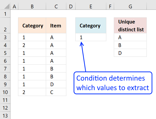
1. VLOOKUP - Return multiple unique distinct values
How to return multiple values using VLOOKUP in Excel and removing duplicates?
I have tried the formula to return multiple values using the index example and worked fine with no duplicate item but how can I list them without the duplicate?
Answer:
The following array formula is easier to understand than a VLOOKUP formula.
Update, 2017-08-16! New smaller regular formula.
Formula in cell G3:
Array formula in cell G3:
The formulas above do not sort the unique distinct list.
1.1 Watch I video where I explain the formula above
Recommended articles
Recommended articles

First, let me explain the difference between unique values and unique distinct values, it is important you know the difference […]
Recommended articles

This post explains how to lookup a value and return multiple values. No array formula required.
Recommended articles
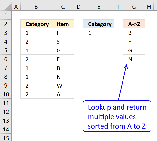
This article demonstrates how to extract multiple values based on a search value and display them sorted from A to […]
1.2 How to enter an array formula
- Double press with left mouse button on cell G3
- Copy (Ctrl + c) and paste (Ctrl + v) array formula to cell
- Press and hold Ctrl + Shift simulatenously
- Press Enter once
- Release all keys
Recommended articles

Array formulas allows you to do advanced calculations not possible with regular formulas.
1.3 Copy array formula
- Select cell G3
- Copy cell ( Ctrl + c)
- Select cell range G4:10
- Paste (Ctrl - v)
1.4 Explaining array formula in cell E8
Step 1 - Compare cell value in E3 with column Category and return a boolean array
The less than and larger than characters are logical operators, they return boolean value TRUE if the condition is met and FALSE if not.
$B$3:$B$10<>$E$3
returns {FALSE; TRUE; FALSE; ... ; TRUE}
Step 2 - Check earlier values above the current cell
The COUNTIF function calculates the number of cells that is equal to a condition.
Function syntax: COUNTIF(range, criteria)
COUNTIF($G$2:G2,$C$3:$C$10)
returns {0;0;0;... ;0}.
Step 3 - Add arrays
The plus sign lets you add numbers in an Excel formula. You can use the plus sign to create OR logic between boolean values or their numerical equivalents.
TRUE - any number except 0 (zero)
FALSE - 0 (zero)
COUNTIF($G$2:G2,$C$3:$C$10)+($B$3:$B$10<>$E$3)
becomes
{FALSE; TRUE; FALSE; FALSE; FALSE; FALSE; FALSE; TRUE} + {0;0;0;0;0;0;0;0}
and returns
{0;1;0;0;0;0;0;1}.
TRUE + TRUE = TRUE
TRUE + FALSE = TRUE
FALSE + FALSE = FALSE
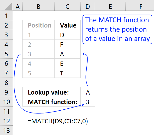
Step 4 - Match first zero value in array and return relative position
The MATCH function returns the relative position of an item in an array that matches a specified value in a specific order.
Function syntax: MATCH(lookup_value, lookup_array, [match_type])
MATCH(0,COUNTIF($G$2:G2,$C$3:$C$10)+($B$3:$B$10<>$E$3),0)
becomes
MATCH(0,{0;1;0;0;0;0;0;1},0)
and returns 1.
Step 5 - Return a value or reference of the cell at the intersection of a particular row and column
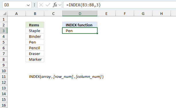
The INDEX function returns a value or reference from a cell range or array, you specify which value based on a row and column number.
Function syntax: INDEX(array, [row_num], [column_num])
INDEX($C$3:$C$10,MATCH(0,COUNTIF($G$2:G2,$C$3:$C$10)+($B$3:$B$10<>$E$3),0))
and returns "A" in cell G3.
Recommended articles
Gets a value in a specific cell range based on a row and column number.
1.5 Get excel file
Vlookup - Return multiple unique distinct valuesv2.xlsx
(Excel 97-2003 Workbook *.xls)
2. VLOOKUP - Return multiple unique distinct values (Excel 365)

Excel 365 dynamic array formula in cell G3:
2.1 Explaining formula
Step 1 - Logical expression
The equal sign is a logical operator, it compares value to value. It also works with value to multiple values. The result is a boolean value TRUE or FALSE.
E3=B3:B10
returns {TRUE; FALSE; TRUE; ... ; FALSE}.
Step 2 - Filter values
The FILTER function extracts values/rows based on a condition or criteria.
Function syntax: FILTER(array, include, [if_empty])
FILTER(C3:C10,E3=B3:B10)
returns {"A";"A";"A";"B";"B";"C"}.
Step 3 - Unique distinct values
The UNIQUE function returns a unique or unique distinct list.
Function syntax: UNIQUE(array,[by_col],[exactly_once])
UNIQUE(FILTER(C3:C10,E3=B3:B10))
returns {"A";"B";"C"}.
3. Create a unique distinct list based on criteria
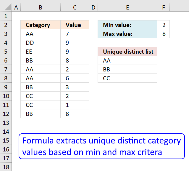
The regular formula in cell E6 extracts unique distinct values from column B based on the corresponding number in column C, the min value is in cell F2 and the Max value is in cell F3.
Formula in cell E6:
Explaining formula in cell E6
Step 1 - Prevent duplicate values
The COUNTIF function counts values based on a condition, in this case, multiple conditions. The first argument has an expanding cell range that grows when the cell is copied to cells below. This allows the formula to count for previously shown values.
COUNTIF($E$5:E5, $B$3:$B$12)=0
returns {TRUE;TRUE;TRUE;... ;TRUE}.
Step 2 - Check which records meet criteria
The less than and greater than signs lets you create logical expressions. Each condition is checked against the values in column C.
($C$3:$C$12<=$F$3)*($C$3:$C$12>=$F$2)
returns {1;0;0;... ;1}
Step 3 - Multiply arrays
All criteria must be met.
(COUNTIF($E$5:E5,$B$3:$B$12)=0)*($C$3:$C$12<=$F$3)*($C$3:$C$12>=$F$2)
returns {1;0;0;... ;1}
Step 4 - Divide 1 with array
The LOOKUP function ignores errors, if we divide something with 0 (zero) we get #DIV/0! error.
1/((COUNTIF($E$5:E5,$B$3:$B$12)=0)*($C$3:$C$12<=$F$3)*($C$3:$C$12>=$F$2))
returns {1;#DIV/0!;... ;1}.
Step 5 - Return value
LOOKUP(2, 1/((COUNTIF($E$5:E5, $B$3:$B$12)=0)*($C$3:$C$12<=$F$3)*($C$3:$C$12>=$F$2)), $B$3:$B$12)
returns "AA"
Get Excel *.xlsx file
unique-list-with-criteria_1v2.xlsx
4. Filter unique distinct values where adjacent cells contain search string
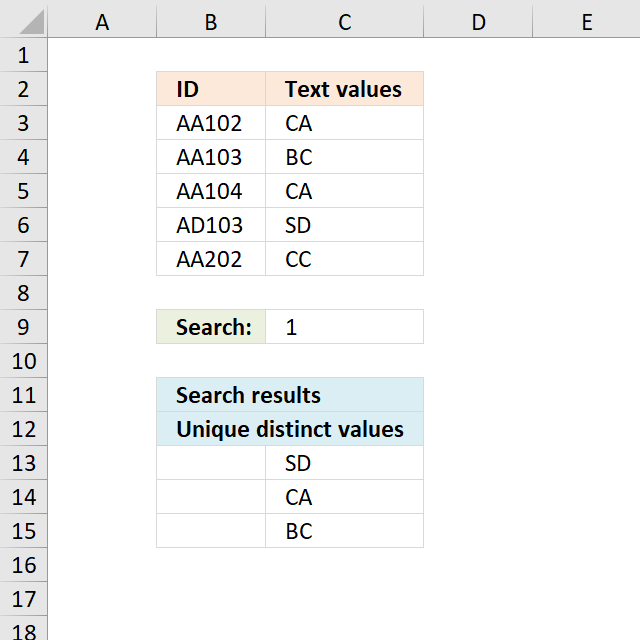
Question: How do I create a unique distinct list where adjacent cell values contain a search string?
AA102 CA
AA103 BC
AA104 CA
AD103 SD
AA201 CC
Search string: 1
Unique distinct list
CA
BC
SD
The formula in cellC13 extracts unique distinct values from cell range C3:C7 if adjacent value in column B contains 1.
Formula in C13:
copied down as far as needed.
Excel 365 dynamic array formula in cell C13:
Explaining formula in cell C13
Step 1 - Identify adjacent values containing the search string
The SEARCH function returns a number representing the position of a given string in a cell.
SEARCH($C$9, $B$3:$B$7)
returns {3; 3; 3; 3; #VALUE!}
Step 2 - Prevent duplicates
The COUNTIF function counts values based on a condition or criteria, if number is 0 (zero) then value has not yet been displayed. The first argument contains an expanding cell reference, when you copy the cell and paste to cells below the cell reference grows. This will make the formula aware of displayed values above current cell.
COUNTIF($C$12:C12, $C$3:$C$7)=0
returns {TRUE; TRUE; TRUE; TRUE; TRUE}.
Step 3 - Multiply arrays
Use AND logic because both arrays must be TRUE in order to be extracted.
((COUNTIF($C$12:C12, $C$3:$C$7)=0)*SEARCH($C$9, $B$3:$B$7))
returns {TRUE; TRUE; TRUE; TRUE; #VALUE!}
Step 4 - Divide 1 with array
Divide 1 with array will return a !DIV/0 error if value is zero or FALSE. Any #VALUE! error will continue as is in array, as well.
1/((COUNTIF($C$12:C12, $C$3:$C$7)=0)*SEARCH($C$9, $B$3:$B$7))
returns {1; 1; 1; 1; #VALUE!}
Step 5 - Get value
The LOOKUP function returns values ignoring error values, the COUNTIF function makes sure that unique distinct values are extracted.
LOOKUP(2, 1/((COUNTIF($C$12:C12, $C$3:$C$7)=0)*SEARCH($C$9, $B$3:$B$7)), $C$3:$C$7)
returns "SD" in cell C13.
Get Excel *.xlsx file
Extract unique distinct values where search string is found in adjacent cells.xlsx
5. Extract unique distinct values from cell range that begins with string
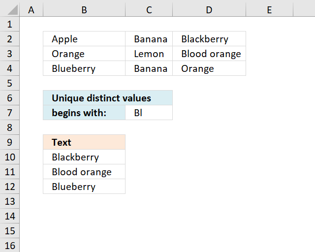
The array formula in cell B10 extracts unique distinct values from cell range B2:D4 that begins with a given condition specified in cell C7.
Excel 365 dynamic array formula in cell B10:
Array formula in B10:
Copy cell B10 and paste it down as far as needed.
Explaining formula in cell B10
Step 1 - Identify values beginning with search string
The LEFT function returns a given number of characters from the start of a text string.
LEFT($B$2:$D$4, LEN($C$7))=$C$7
returns {FALSE,FALSE,TRUE; ... ,FALSE}.
Step 2 - Keep track of previous values
The COUNTIF function counts values based on a condition or criteria, the first argument contains an expanding cell reference, it grows when the cell is copied to cells below. This makes the formula aware of values displayed in cells above.
COUNTIF(B9:$B$9, $B$2:$D$4)=0
returns {TRUE,TRUE,TRUE; ... ,TRUE}.
Step 3 - Multiply arrays
Both values must be true in order to get the value in a later step.
(LEFT($B$2:$D$4, LEN($C$7))=$C$7)*(COUNTIF(B9:$B$9, $B$2:$D$4)=0)
returns {0,0,1; ... ,0}
Step 4 - Replace TRUE with unique number
The IF function returns a unique number if boolean value is TRUE. FALSE returns "" (nothing). The unique number is needed to find the right value in a later step.
IF((LEFT($B$2:$D$4, LEN($C$7))=$C$7)*(COUNTIF(B9:$B$9, $B$2:$D$4)=0), (ROW($B$2:$D$4)+(1/(COLUMN($B$2:$D$4)+1)))*1, "")
returns {"","",2.2;... ,""}
Step 5 - Find smallest value in array
The MIN function returns the smallest number in array ignoring blanks and text values.
MIN(IF((LEFT($B$2:$D$4,LEN($C$7))=$C$7)*(COUNTIF(B9:$B$9, $B$2:$D$4)=0), (ROW($B$2:$D$4)+(1/(COLUMN($B$2:$D$4)+1)))*1, ""))
returns 2.2.
Step 6 - Find corresponding value
IF(MIN(IF((LEFT($B$2:$D$4, LEN($C$7))=$C$7)*(COUNTIF(B9:$B$9, $B$2:$D$4)=0), (ROW($B$2:$D$4)+(1/(COLUMN($B$2:$D$4)+1)))*1, ""))=(ROW($B$2:$D$4)+(1/(COLUMN($B$2:$D$4)+1)))*1, $B$2:$D$4, "")
returns {"","","Blackberry";"","","";"","",""}
Step 7 - Concatenate strings in array
The TEXTJOIN function returns values concatenated ignoring blanks in array.
TEXTJOIN("", TRUE, IF(MIN(IF((LEFT($B$2:$D$4, LEN($C$7))=$C$7)*(COUNTIF(B9:$B$9, $B$2:$D$4)=0), (ROW($B$2:$D$4)+(1/(COLUMN($B$2:$D$4)+1)))*1, ""))=(ROW($B$2:$D$4)+(1/(COLUMN($B$2:$D$4)+1)))*1, $B$2:$D$4, ""))
returns "Blackberry" in cell B10.
Get Excel *.xlsx file
Extract unique distinct values begins with A in a range using array formula in excel.xlsx
6. Extract unique distinct text values containing string in a range
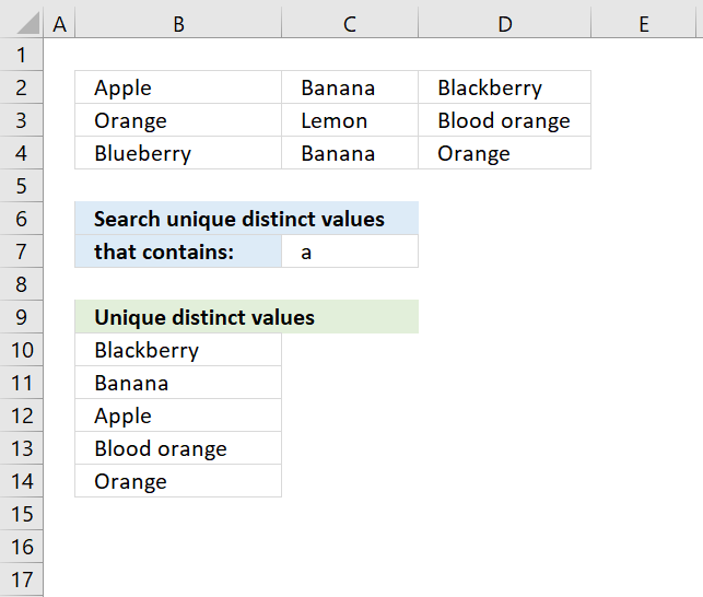
The formula in cell B10 extracts unique distinct values from cell range B2:d4 that contains the string specified in cell C7.
Excel 365 dynamic array formula in cell B10:
Array formula in B10:
To enter an array formula, type the formula in a cell then press and hold CTRL + SHIFT simultaneously, now press Enter once. Release all keys.
The formula bar now shows the formula with a beginning and ending curly bracket telling you that you entered the formula successfully. Don't enter the curly brackets yourself.
Explaining formula in cell B10
Step 1 - Identify values containing search string
The SEARCH function returns a number representing the location of a text string in another string.
ISNUMBER(SEARCH($C$7,$B$2:$D$4))
returns {TRUE,TRUE, TRUE;... , TRUE}
Step 2 - Keep track of previous values
The COUNTIF function counts values based on a condition or criteria, the first argument contains an expanding cell reference, it grows when the cell is copied to cells below. This makes the formula aware of values displayed in cells above. 0 (zero) indicates values that not yet have been displayed
COUNTIF(B9:$B$9,$B$2:$D$4)=0
returns {TRUE,TRUE,TRUE; ... ,TRUE}.
Step 3 - Multiply arrays
Both values must be true in order to get the value in a later step.
(COUNTIF(B9:$B$9,$B$2:$D$4)=0)*ISNUMBER(SEARCH($C$7,$B$2:$D$4))
returns {1,1,1;..., 1}
Step 4 - Replace TRUE with unique number
The IF function returns a unique number if boolean value is TRUE. FALSE returns "" (nothing). The unique number is needed to find the right value in a later step.
IF((COUNTIF(B9:$B$9,$B$2:$D$4)=0)*ISNUMBER(SEARCH($C$7,$B$2:$D$4)),(ROW($B$2:$D$4)+(1/(COLUMN($B$2:$D$4)+1)))*1,"")
returns {2.33333333333333, 2.25,2.2; .... , 4.2}
Step 5 - Find smallest value in array
The MIN function returns the smallest number in array ignoring blanks and text values.
MIN(IF((COUNTIF(B9:$B$9,$B$2:$D$4)=0)*ISNUMBER(SEARCH($C$7,$B$2:$D$4)),(ROW($B$2:$D$4)+(1/(COLUMN($B$2:$D$4)+1)))*1,""))
returns 2.2.
Step 6 - Find corresponding value
IF(MIN(IF((COUNTIF(B9:$B$9,$B$2:$D$4)=0)*ISNUMBER(SEARCH($C$7,$B$2:$D$4)),(ROW($B$2:$D$4)+(1/(COLUMN($B$2:$D$4)+1)))*1,""))=(ROW($B$2:$D$4)+(1/(COLUMN($B$2:$D$4)+1)))*1,$B$2:$D$4,"")
returns {"","","Blackberry";"","","";"","",""}
Step 7 - Concatenate strings in array
The TEXTJOIN function returns values concatenated ignoring blanks in array.
TEXTJOIN("",TRUE,IF(MIN(IF((COUNTIF(B9:$B$9,$B$2:$D$4)=0)*ISNUMBER(SEARCH($C$7,$B$2:$D$4)),(ROW($B$2:$D$4)+(1/(COLUMN($B$2:$D$4)+1)))*1,""))=(ROW($B$2:$D$4)+(1/(COLUMN($B$2:$D$4)+1)))*1,$B$2:$D$4,""))
returns "Blackberry" in cell B10.
Get Excel *.xlsx
Filter unique distinct text values containing string in a range.xlsx
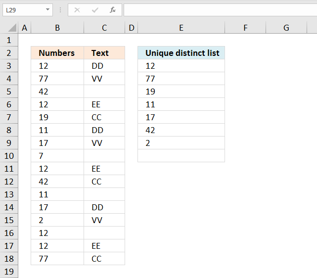
7. Extract unique distinct values if adjacent cell is text
Array formula in D3:
Excel 365 dynamic array formula in cell D3:
How to create an array formula
- Copy array formula (Ctrl + c)
- Double press with left mouse button on cell D2
- Paste array formula (Ctrl + v)
- Press and hold Ctrl + Shift
- Press Enter
Recommended article
Recommended articles
Array formulas allows you to do advanced calculations not possible with regular formulas.
Explaining formula in cell D3
Step 1 - Check if adjacent values are not text values
The ISTEXT function returns boolean value TRUE if a cell contains a text value and FALSE if not. I am using a cell range as an argument so the function returns an array of bollean values.
They correspond to the input values based on position. The image below shows the array from ISTEXT($B$2:$B$17)
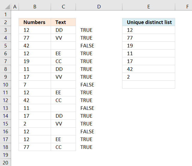
We need to know which values are not text values, the array is compared to boolean value FALSE. This will change TRUE to FALSE and FALSE top TRUE, the array becomes:
The image below shows the array from ISTEXT($B$2:$B$17)=FALSE
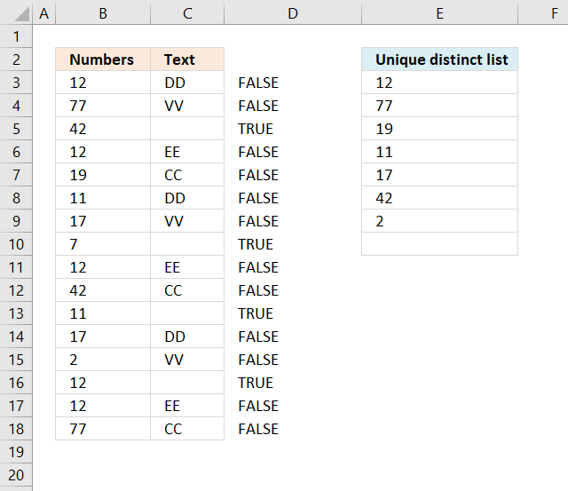
Excel handles FALSE as the same as 0 (zero) and TRUE as 1 or more.
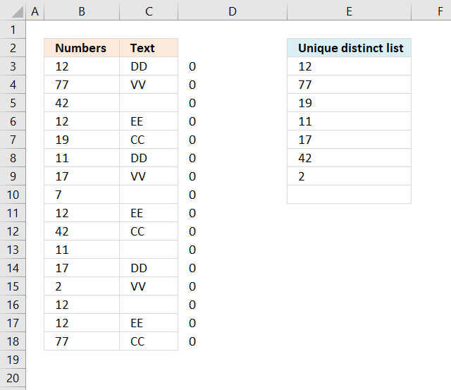
Step 2 - Check if value is unique
The COUNTIF function counts values based on a condition or multiple conditions. It has two arguments range and criteria. The first argument is a cell reference that grows when cell is copied to cell below.
It contains a cell reference with two parts, the first one is absolute and the second is a relative cell reference. The COUNTIF function is most often used to return a single value, however, in this case, we need it to return an array of values that match the relative positions of the cell values.
COUNTIF($D$1:D1, $A$2:$A$17)
No values have been displayed yet so the array contains 0 (zeros) , if a value had been 1 or more it would have indicated that the value has been displayed in a cell above the current cell.
The image below shows the array in column D.
The image below shows the array in column D from COUNTIF($D$1:D1, $A$2:$A$17)+(ISTEXT($B$2:$B$17)=FALSE)
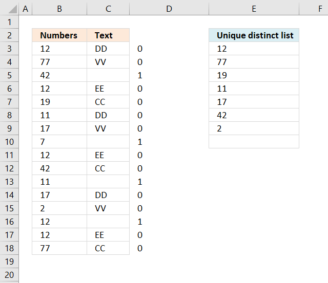
This array tells us which values that have not yet been displayed and where the adjacent value is a text value.
Recommended articles

Counts the number of cells that meet a specific condition.
Step 3 - Find relative position
The MATCH function identifies the position of the first cell value that has not yet been shown and where the adjacent value is a text value.
It matches an exact match meaning a value that is exactly equal to 0 (zer0), this is determined by the third argument.
MATCH(0, COUNTIF($D$1:D1, $A$2:$A$17)+(ISTEXT($B$2:$B$17)=FALSE), 0)
returns 1.
The MATCH function has identified the first value in the array as a unique distyinct value that has an adjacent cell value that contains a text value.
Recommended articles
Identify the position of a value in an array.
Step 4 - Return value
The INDEX function simply returns a value from a cell range based on a row and column coordinate. The column coordinate is not neccessary since this example has all values in a single column.
INDEX($A$2:$A$17, MATCH(0, COUNTIF($D$1:D1, $A$2:$A$17)+(ISTEXT($B$2:$B$17)=FALSE), 0))
returns 12 in cell D3.
Recommended articles
Gets a value in a specific cell range based on a row and column number.
Get the Excel file
unique-list-to-be-created-from-a-column-where-an-adjacent-column-has-text-cell-values3.xlsx
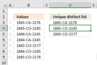
8. Extract unique distinct values based on the 4 last characters
The good thing about this formula is that it is short and easy to remember. The main drawback with countif is that it is not able to coerce a range.
I would like an unique list based on the last 4 characters in a cell. This would mean using the right function.
1845-CA-2176
1845-CO-2145
1846-CA-2145
The unique list here is 2145 and 2176.
Is there a short but sweet formula like the original countif formula above?
The following formula will not work with countif- =TEXT(A1:A3,mmmmyy).
Answer:
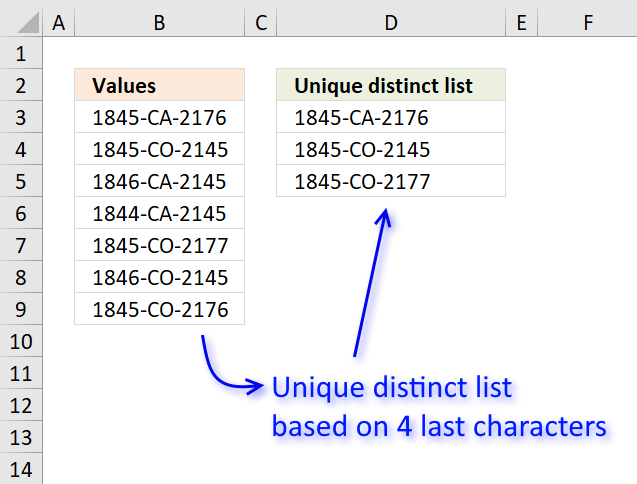
The picture above shows an array formula in cell D3 that extracts a unique distinct list based on the four last characters in the cell value.
You can easily replace the RIGHT function with LEFT or MID function to get a unique distinct list based on other criteria.
The issue here is that the first argument in the COUNTIF function won't accept anything else than a cell range. Not even an array of constants will work.
There are exceptions o this rule, you can use the OFFSET function in the first argument, however that won't be much help in this case.
To enter an array formula, type the formula in cell B3 then press and hold CTRL + SHIFT simultaneously, now press Enter once. Release all keys.
 The formula bar now shows the formula with a beginning and ending curly bracket telling you that you entered the formula successfully.
Don't enter the curly brackets yourself, they appear automatically.
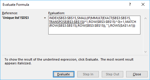
Explaining formula in cell D3
Use "Evaluate Formula" on tab "Formula" on the ribbon to go through the formula in small steps.
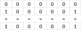
Step 1 - Compare previous values with source list
This step compares previous values above the current cell with the source list.
This makes the formula extract only unique distinct values, the RIGHT function extracts the four last characters in each cell.
RIGHT($D$2:D2, 4)=TRANSPOSE(RIGHT($B$3:$B$9, 4))
becomes
"list"={"2176", "2145", "2145", "2145", "2177", "2145", "2176"}
returns
{FALSE, FALSE, FALSE, FALSE, FALSE, FALSE, FALSE}
![]()
Remember that in cell D3 there are no previous values except the header value.
$D$2:D2 is an absolute and relative cell reference. This makes it expand as the formula is copied to cells below. Make sure to copy the cell, not the formula.
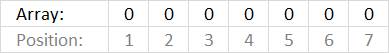
Step 2 - Sum values column-wise
The formula needs to know which values have been displayed and which has not. It returns an array with the same size as the source list, 1 indicates that the value has been shown and 0 (zero) indicates it has not been shown.
The MMULT function is able to sum array values column-wise or row-wise depending on how you use it, you need two arguments in the MMULT function. Read more about the MMULT function here.
MMULT(TRANSPOSE(ROW($A$1:A1)^0), (RIGHT($D$2:D2, 4)=TRANSPOSE(RIGHT($B$3:$B$9, 4)))*1)
becomes
MMULT(1, ({FALSE, FALSE, FALSE, FALSE, FALSE, FALSE, FALSE})*1)
becomes
MMULT(1, {0, 0, 0, 0, 0, 0, 0}))
and returns {0, 0, 0, 0, 0, 0, 0}.
This array tells the formula that all values can be extracted in cell D3, in other words no value in the source list have been displayed in cells above yet.
The calculation seems pointless in cell D3, however, it uses a cell reference that expands so the array becomes more and more advanced in cells further down.
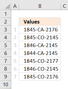
 For example, in cell D4 the array becomes:
MMULT({1,1},{0,0,0,0,0,0,0;1,0,0,0,0,0,1})
and returns {1,0,0,0,0,0,1}.
 The array tells the formula not to get the first and last value in cell range B3:B9 because 1845-CA-2176 has been displayed in D3.
1845-CA-2176 and 1845-CO-2176 share the same last four characters.
The picture to the right shows the array next to cell values in B3:B9.
Step 3 - Identify position of the first 0 (zero) in array
The MATCH function returns the relative position of a given value in an array or cell range.
MATCH(0, MMULT(TRANSPOSE(ROW($A$1:A1)^0), (RIGHT($D$2:D2, 4)=TRANSPOSE(RIGHT($B$3:$B$9, 4)))*1), 0)
becomes
MATCH(0, {0,0,0,0,0,0,0}, 0)
and returns 1.
Remember that this is for cell D3.
If we continue with the formula in cell D4:
MATCH(0, {1,0,0,0,0,0,1}, 0)
and returns 2. The first 0 (zero) in the array is in position 2.
Step 4 - Return value in given position
The formula in cell D3 is:
INDEX($B$3:$B$9, MATCH(0, MMULT(TRANSPOSE(ROW($A$1:A1)^0), (RIGHT($D$2:D2, 4)=TRANSPOSE(RIGHT($B$3:$B$9, 4)))*1), 0))
 becomes
INDEX($B$3:$B$9, 1)
and returns the value in $B$3 which is 1845-CA-2176 to cell D3.
If we move on to cell D4 the formula is:
INDEX($B$3:$B$9, 2)
and returns the value in cell $B$4 to cell D4 which is 1845-CO-2145.
Get Excel *.xlsx file
![]() Filter unique distinct strings within a cell.xlsx
Filter unique distinct strings within a cell.xlsx
9. Remove duplicates within same month or year
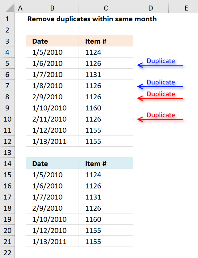
The array formula in cell B15 extracts dates from B4:B12 if it is not a duplicate item in the same month and year.
Excel 365 dynamic array formula in cell B15:
Array formula in B15:
To enter an array formula, type the formula in a cell then press and hold CTRL + SHIFT simultaneously, now press Enter once. Release all keys.
The formula bar now shows the formula with a beginning and ending curly bracket telling you that you entered the formula successfully. Don't enter the curly brackets yourself.
Array formula in C15:
Explaining formula in cell B15
Step 1 - Concatenate year, month and item value
The YEAR function returns the year of an Excel date, the MONTH function returns the MONTH of an Excel date.
YEAR($B$4:$B$12)&"-"&MONTH($B$4:$B$12)&"-"&$C$4:$C$12
becomes
YEAR({40183; 40184; 40185; 40186; 40218; 40188; 40220; 40190; 40556})&"-"&MONTH({40183; 40184; 40185; 40186; 40218; 40188; 40220; 40190; 40556})&"-"&{1124; 1126; 1131; 1126; 1126; 1160; 1126; 1155; 1155}
The & ampersand sign lets you concatenate values, in this case, row-wise.
YEAR({40183; 40184; 40185; 40186; 40218; 40188; 40220; 40190; 40556})&"-"&MONTH({40183; 40184; 40185; 40186; 40218; 40188; 40220; 40190; 40556})&"-"&{1124; 1126; 1131; 1126; 1126; 1160; 1126; 1155; 1155}
returns
{"2010-1-1124"; "2010-1-1126"; "2010-1-1131"; "2010-1-1126"; "2010-2-1126"; "2010-1-1160"; "2010-2-1126"; "2010-1-1155"; "2011-1-1155"}
Step 2 - Match concatenated values to identify duplicates
The MATCH function finds the relative position of a value in an array or cell range.
MATCH(YEAR($B$4:$B$12)&"-"& MONTH($B$4:$B$12)&"-"&$C$4:$C$12, YEAR($B$4:$B$12)& "-"&MONTH($B$4:$B$12)& "-"&$C$4:$C$12, 0)
becomes
MATCH{"2010-1-1124"; "2010-1-1126"; "2010-1-1131"; "2010-1-1126"; "2010-2-1126"; "2010-1-1160"; "2010-2-1126"; "2010-1-1155"; "2011-1-1155"}, {"2010-1-1124"; "2010-1-1126"; "2010-1-1131"; "2010-1-1126"; "2010-2-1126"; "2010-1-1160"; "2010-2-1126"; "2010-1-1155"; "2011-1-1155"}, 0)
and returns
{1; 2; 3; 2; 5; 6; 5; 8; 9}
Step 3 - Compare value to sequence
If number is equal to corresponding number in sequence the logical expression returns TRUE.
MATCH(YEAR($B$4:$B$12)&"-"& MONTH($B$4:$B$12)&"-"& $C$4:$C$12,YEAR($B$4:$B$12)&"-"& MONTH($B$4:$B$12)&"-"& $C$4:$C$12,0)=MATCH(ROW($B$4:$B$12), ROW($B$4:$B$12))
becomes
{1; 2; 3; 2; 5; 6; 5; 8; 9}=MATCH(ROW($B$4:$B$12), ROW($B$4:$B$12))
becomes
{1; 2; 3; 2; 5; 6; 5; 8; 9}={1;2;3;4;5;6;7;8;9}
and returns
{TRUE; TRUE; TRUE; FALSE; TRUE; TRUE; FALSE; TRUE; TRUE}
Step 4 - Replace TRUE with corresponding row number
The IF function has three arguments, the first one must be a logical expression. If the expression evaluates to TRUE then one thing happens (argument 2) and if FALSE another thing happens (argument 3).
IF(MATCH(YEAR($B$4:$B$12)&"-"&MONTH($B$4:$B$12)&"-"&$C$4:$C$12, YEAR($B$4:$B$12)&"-"&MONTH($B$4:$B$12)&"-"&$C$4:$C$12, 0)=MATCH(ROW($B$4:$B$12), ROW($B$4:$B$12)), MATCH(ROW($B$4:$B$12), ROW($B$4:$B$12)), "")
becomes
IF({TRUE; TRUE; TRUE; FALSE; TRUE; TRUE; FALSE; TRUE; TRUE}=MATCH(ROW($B$4:$B$12), ROW($B$4:$B$12)), MATCH(ROW($B$4:$B$12), ROW($B$4:$B$12)), "")
becomes
IF({TRUE; TRUE; TRUE; FALSE; TRUE; TRUE; FALSE; TRUE; TRUE}, {1;2;3;4;5;6;7;8;9}, "")
and returns
{1;2;3;"";5;6;"";8;9}.
Step 5 - Extract k-th smallest row number
To be able to return a new value in a cell each I use the SMALL function to filter column numbers from smallest to largest.
The ROWS function keeps track of the numbers based on an expanding cell reference. It will expand as the formula is copied to the cells below.
SMALL(IF(MATCH(YEAR($B$4:$B$12)&"-"&MONTH($B$4:$B$12)&"-"&$C$4:$C$12, YEAR($B$4:$B$12)&"-"&MONTH($B$4:$B$12)&"-"&$C$4:$C$12, 0)=MATCH(ROW($B$4:$B$12), ROW($B$4:$B$12)), MATCH(ROW($B$4:$B$12), ROW($B$4:$B$12)), ""), ROWS($A$1:A1))
becomes
SMALL({1;2;3;"";5;6;"";8;9}, ROWS($A$1:A1))
becomes
SMALL({1;2;3;"";5;6;"";8;9}, 1)
and returns 1.
Step 6 - Get value
The INDEX function returns a value based on a cell reference and column/row numbers.
INDEX($C$4:$C$12, SMALL(IF(MATCH(YEAR($B$4:$B$12)&"-"&MONTH($B$4:$B$12)&"-"&$C$4:$C$12, YEAR($B$4:$B$12)&"-"&MONTH($B$4:$B$12)&"-"&$C$4:$C$12, 0)=MATCH(ROW($B$4:$B$12), ROW($B$4:$B$12)), MATCH(ROW($B$4:$B$12), ROW($B$4:$B$12)), ""), ROWS($A$1:A1)))
becomes
INDEX($C$4:$C$12, 1)
and returns 1/5/2010 in cell B15.
Get Excel *.xlsx file
Remove-duplicates-in-same-month.xlsx
Remove duplicates within same year in excel

Array formula in B38:
Array formula in C38:
Get excel sample file for this article.
Remove-duplicates-in-same-month.xls
(Excel 97-2003 Workbook *.xls)
10. Filter unique distinct values based on a date range

The image above shows a formula in cell E6 that extracts unique distinct values if the corresponding dates match the date range specified in cells F2 and F3.
The date range is specified in cell G1 and G2, see image above.
Array formula in cell D2:
10.1 How to enter an array formula
To enter an array formula, type the formula in a cell then press and hold CTRL + SHIFT simultaneously, now press Enter once. Release all keys.
The formula bar now shows the formula with a beginning and ending curly bracket telling you that you entered the formula successfully. Don't enter the curly brackets yourself.

10.2 Explaining the formula in cell D2
Step 1 - Which dates are later than or equal to the start date?
The less than sign and equal sign are logical operators, they allow you to compare numbers and text strings. The result are boolean values and is either TRUE or FALSE.
$F$3>=$C$3:$C$18 returns {TRUE; FALSE; ... ; TRUE}.
Step 2 - Which dates are earlier than or equal to the end date?
$F$2<=$C$3:$C$18 returns {TRUE; TRUE; ... ; TRUE}.
Step 3 - AND logic
We need to identify dates that meet both conditions, we can do that by multiplying the arrays. The parentheses allow us to control the order of operation.
($F$3>=$C$3:$C$18)*($F$2<=$C$3:$C$18) returns {1; 0; 0; ... ; 1}.
Step 4 - Replace 1 with the corresponding number on the same row
The IF function returns one value if the logical test is TRUE and another value if the logical test is FALSE.
IF(logical_test, [value_if_true], [value_if_false])
IF(($F$3>=$C$3:$C$18)*($F$2<=$C$3:$C$18), $B$3:$B$18, $E$5)
returns {12; "Unique distinct values"; ... ; 77}.
Step 5 - Count previous displayed values
The COUNTIF function calculates the number of cells that is equal to a condition.
COUNTIF(range, criteria)
COUNTIF($E$5:E5, IF(($F$3>=$C$3:$C$18)*($F$2<=$C$3:$C$18), $B$3:$B$18, $E$5))
returns {0; 1; 1; ... ; 0}.
Step 6 - Find first not displayed values in array
The MATCH function returns the relative position of an item in an array or cell reference that matches a specified value in a specific order.
MATCH(lookup_value, lookup_array, [match_type])
MATCH(0,COUNTIF($E$5:E5, IF(($F$3>=$C$3:$C$18)*($F$2<=$C$3:$C$18), $B$3:$B$18, $E$5)), 0) returns 1.
Step 7 - Get value
The INDEX function returns a value from a cell range, you specify which value based on a row and column number.
INDEX(array, [row_num], [column_num], [area_num])
INDEX($B$3:$B$18, MATCH(0,COUNTIF($E$5:E5, IF(($F$3>=$C$3:$C$18)*($F$2<=$C$3:$C$18), $B$3:$B$18, $E$5)), 0)) returns 12 in cell E6.
Step 8 - Remove error values
The IFERROR function handles error values which the formula returns when no more values can be displayed.
IFERROR(INDEX($B$3:$B$18, MATCH(0,COUNTIF($E$5:E5, IF(($F$3>=$C$3:$C$18)*($F$2<=$C$3:$C$18), $B$3:$B$18, $E$5)), 0)), "")
11. Filter unique distinct values based on a date range (Excel 365)

Dynamic array formula in cell E6:
11.1 How to enter a dynamic array formula
The dynamic array formula is a new feature in Excel 365, you enter it as a regular formula.
11.2 Explaining dynamic array formula
Step 1 - Find dates earlier than or equal to end date
The less than sign and equal sign are logical operators, they allow you to compare numbers and text strings. The result is boolean values and the result is either TRUE or FALSE.
C3:C18<=F3 returns {TRUE; FALSE; ... ; TRUE}
Step 2 - Find dates later than or equal to start date
C3:C18>=F2 returns {TRUE; TRUE; ... ; TRUE}.
Step 3 - AND logic
Both tests must evaluate to true and to do that we need to multiply the array, in other words, apply AND logic.
Use the asterisk to multiply values or arrays.
* (asterisk) - Both logical expressions must match (AND logic)
The AND logic behind this is that
TRUE * TRUE = TRUE (1)
TRUE * FALSE = FALSE (0)
FALSE * FALSE = FALSE (0)
The parentheses control the order of operation.
(C3:C18<=F3)*(C3:C18>=F2)
returns {1; 0; ... ; 1}.
Step 4 - Filter values based on conditions
The FILTER function lets you extract values/rows based on a condition or criteria. It is in the Lookup and reference category and is only available to Excel 365 subscribers.
FILTER(array, include, [if_empty])
FILTER(B3:B18, (C3:C18<=F3)*(C3:C18>=F2)) returns {12; 77; 17; 7; 12; 12; 77}.
Step 5 - Extract unique distinct values based on array
The UNIQUE function lets you extract both unique and unique distinct values and also compare columns to columns or rows to rows.
UNIQUE(array,[by_col],[exactly_once])
UNIQUE(FILTER(B3:B18, (C3:C18<=F3)*(C3:C18>=F2))) returns {12; 77; 17; 7}.
Get Excel file
Get the Excel file
unique-list-to-be-created-from-a-column-where-an-adjacent-column-is-in-a-date-range.xlsx
12. Extract unique distinct values if the value contains a given string - Excel 365
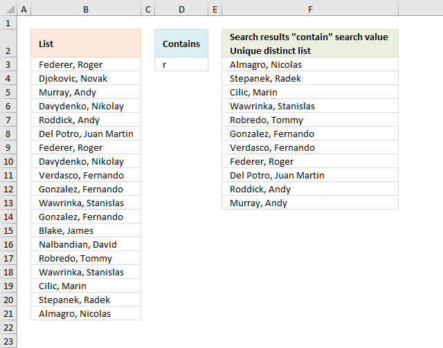
The following formula lists unique distinct values from cell range B3:B21 if they contain the substring specified in cell D3. Unique distinct values are all values except duplicates, they are merged into one distinct value.
The image above shows names in cell range B3:B21, the sub string is specified in cell D3 and the result is displayed in cells F3:F13. The result is an dynamic array that spills to adjacent cells below automatically.
Excel 365 formula in cell F3:
The result is an array containing names from source range B3:B21 that contains "r".
Okay, let's go through the formula step by step, starting with the innermost function:
- SEARCH(D3, B3:B21): The SEARCH function searches for the value in cell D3 within each cell in the range B3:B21. It returns the starting position of the first occurrence of the value in D3 within the corresponding cell in B3:B21. If the value in D3 is not found in a cell, the SEARCH function returns 0 (zero).
- ISNUMBER(SEARCH(D3, B3:B21)): The ISNUMBER function checks if the result of the SEARCH function is a number. If the SEARCH function returns a number (i.e., the value in D3 was found in the corresponding cell in B3:B21), the ISNUMBER function will return TRUE. If the SEARCH function returns 0 (i.e., the value in D3 was not found in the corresponding cell in B3:B21), the ISNUMBER function will return FALSE.
- FILTER(B3:B21, ISNUMBER(SEARCH(D3, B3:B21))): The FILTER function takes two arguments: the range to filter (B3:B21) and the condition to apply (ISNUMBER(SEARCH(D3, B3:B21))). The FILTER function creates a new array that contains only the cells from B3:B21 where the corresponding condition (the result of ISNUMBER(SEARCH(D3, B3:B21))) is TRUE. In other words, the FILTER function creates a new array that contains only the cells from B3:B21 where the value in D3 was found.
- UNIQUE(FILTER(B3:B21, ISNUMBER(SEARCH(D3, B3:B21)))): The UNIQUE function takes the array returned by the FILTER function and removes any duplicate values, leaving only the unique values. The final result of this formula is an array containing the unique values from the range B3:B21 where the value in D3 was found.
In summary, the formula first searches for the value in D3 within each cell in the range B3:B21, then filters the range to include only the cells where the value in D3 was found, and finally, it removes any duplicate values from the filtered array, leaving only the unique values.
Explaining formula
Step 1 - Search for a substring in the array
The SEARCH function returns the number of the character at which a specific character or text string is found reading left to right (not case-sensitive)
Function syntax: SEARCH(find_text,within_text, [start_num])
SEARCH(D3, B3:B21)
returns {5; #VALUE!; ... ; 6}.
Step 2 - Check if the value is a number
The ISNUMBER function checks if a value is a number, returns TRUE or FALSE.
Function syntax: ISNUMBER(value)
ISNUMBER(SEARCH(S20,R20:R22))
returns {TRUE; FALSE; T... ; TRUE}.
Step 3 - Filter values if the value in the array is a number
The FILTER function extracts values/rows based on a condition or criteria.
Function syntax: FILTER(array, include, [if_empty])
FILTER(B3:B21,ISNUMBER(SEARCH(S20,R20:R22)))
returns {"Federer, Roger "; "Murray, Andy "; ... ; "Almagro, Nicolas "}.
Step 3 - List unique distinct values
The UNIQUE function returns a unique or unique distinct list.
Function syntax: UNIQUE(array,[by_col],[exactly_once])
UNIQUE(FILTER(B3:B21,ISNUMBER(SEARCH(D3,B3:B21))))
returns {"Federer, Roger "; "Murray, Andy "; ... ; "Almagro, Nicolas "}
13. Extract unique distinct values if the value contains a string in earlier Excel versions
The image above demonstrates a formula in cell F3 that extracts unique distinct values from column B if they contain the value in cell D3. This fomrula worksin all Excel versions, however, you need to enter the formula as an array formula and copy cell F3 to cells below in order to ignore duplicate values.
Formula in cell F3:
Important! The use of absolute cell references in this formula is crucial because it ensures that the formula will work correctly when copied to cells below. If the references were relative the formula would not be able to correctly identify the appropriate ranges and cell references, leading to incorrect results.
This formula is different from the Excel 365 formula above in that it calculates a new value in each cell, whereas the Excel 365 calculates an array and spills the values to cells below. This spilling behavior is new to Excel 365 and doesn't work in earlier Excel versions.
Let's break down this formula step by step:
- COUNTIF($F$2:F2, $B$3:$B$21)=0: The COUNTIF function counts the number of times the value in each cell of the range $B$3:$B$21 appears in the range $F$2:F2. Note that $F$2:F2 id dependent on where you enter the formula and it expands when the formula is copied to cells below. The result of this function is an array of 1s and 0s, where 1 indicates that the value in the corresponding cell of $B$3:$B$21 is found in $F$2:F2, and 0 indicates that the value is not found. The =0 part of the formula checks if the result of COUNTIF is 0, which means the value in the corresponding cell of $B$3:$B$21 is not found in $F$2:F2.
- SEARCH($D$3, $B$3:$B$21): The SEARCH function searches for the value in cell $D$3 within each cell in the range $B$3:$B$21. It returns the starting position of the first occurrence of the value in $D$3 within the corresponding cell in $B$3:$B$21. If the value in $D$3 is not found in a cell, the SEARCH function returns an error value #VALUE!.
- (COUNTIF($F$2:F2, $B$3:$B$21)=0)*SEARCH($D$3, $B$3:$B$21): This part of the formula multiplies the array of 1s and 0s (from the COUNTIF function) with the array of search results (from the SEARCH function). The result is an array where the values are either 0 (if the value in the corresponding cell of $B$3:$B$21 is found in $F$2:F2) or the search result (if the value in the corresponding cell of $B$3:$B$21 is not found in $F$2:F2).
- 1/((COUNTIF($F$2:F2, $B$3:$B$21)=0)*SEARCH($D$3, $B$3:$B$21)): This part of the formula divides 1 by the array created in the previous step. The result is an array where the values are either 1/0 or error (if the value in the corresponding cell of $B$3:$B$21 is found in $F$2:F2) or 1/the search result (if the value in the corresponding cell of $B$3:$B$21 is not found in $F$2:F2). Dividing 1/0 returns #DIV/0 error which the LOOKUP function ignores in the next step below.
- LOOKUP(2, 1/((COUNTIF($F$2:F2, $B$3:$B$21)=0)*SEARCH($D$3, $B$3:$B$21)), $B$3:$B$21): The LOOKUP function takes three arguments: the value to search for (in this case, 2), the array to search in (the array created in the previous step), and the array to return the corresponding values from (the range $B$3:$B$21). The LOOKUP function finds the largest value in the array that is less than or equal to 2, and then returns the corresponding value from the range $B$3:$B$21. The LOOKUP function ignore errors automatically.
Explaining formula in cell F3
These steps shows the results in greater detail.
Step 1 - Prevent duplicates
The COUNTIF function counts cells in cell range based on a condition or criteria. If the value is equal to 0 then it has not been displayed yet.
COUNTIF($F$2:F2, $B$3:$B$21)=0
returns {TRUE; TRUE; ... ; TRUE}
Step 2 - Check if values contain string
The SEARCH function returns a number that represents the position of the search string if found. The function returns an error if not found which is alright in this case.
SEARCH($D$3,$B$3:$B$21)
returns {5; #VALUE!; ... ; 6}.
Step 3 - Multiply arrays
Both values must be TRUE in order to be TRUE meaning if the value has not been displayed yet AND the value contains the string then return TRUE or the equivalent numerical number. TRUE is all numbers except 0 (zero), FALSE is 0 (zero).
returns {5; #VALUE!; ... ; 6}.
Step 4 - Divide 1 with array
The result will return !DIV/0 error if 1 is divided with 0 (0), which the LOOKUP function ignores. It will also ignore #VALUE! errors.
1/((COUNTIF($F$2:F2, $B$3:$B$21)=0)*SEARCH($D$3, $B$3:$B$21))
returns {0.2; #VALUE!;... ; 0.166666666666667}.
Step 5 - Return value
LOOKUP(2,1/((COUNTIF($F$2:F2,$B$3:$B$21)=0)*SEARCH($D$3,$B$3:$B$21)),$B$3:$B$21)
returns "Almagro, Nicolas " in cell F3.
Get Excel *.xlsx file
Filter unique distinct values containing string.xlsx
Unique distinct values category
First, let me explain the difference between unique values and unique distinct values, it is important you know the difference […]
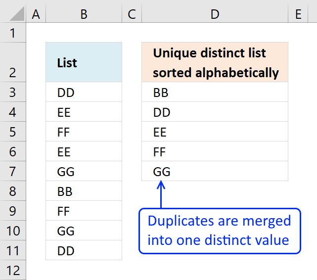
This article demonstrates Excel formulas that allows you to list unique distinct values from a single column and sort them […]
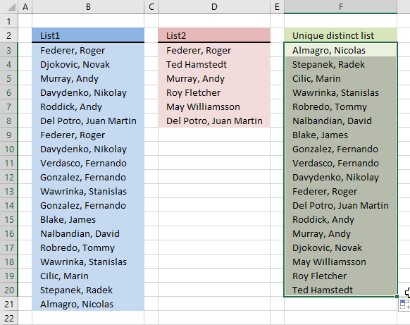
Question: I have two ranges or lists (List1 and List2) from where I would like to extract a unique distinct […]
Excel categories
97 Responses to “VLOOKUP – Return multiple unique distinct values”
Leave a Reply
How to comment
How to add a formula to your comment
<code>Insert your formula here.</code>
Convert less than and larger than signs
Use html character entities instead of less than and larger than signs.
< becomes < and > becomes >
How to add VBA code to your comment
[vb 1="vbnet" language=","]
Put your VBA code here.
[/vb]
How to add a picture to your comment:
Upload picture to postimage.org or imgur
Paste image link to your comment.
can you do this with multiple search strings?
Arielle,
Yes!
Formula in cell C12:
=INDEX(Column_txt, MATCH(0, COUNTIF($C$11:C11, Column_txt)*(ISNUMBER(SEARCH($C$8, Search_column))+ISNUMBER(SEARCH($C$9, Search_column))), 0)) + CTRL + SHIFT + ENTER
Copy cell C12 and paste it down as far as needed.
The second search string is in cell C9.
Okay I need to do this with text that searches cells with text separated by commas.
ex. search string: fin
search string: pro
search string: crm
cell A1: fin, pro, crm
cell A2: pro, crm
will the formula work for that so that it displays the cell that contains all three strings?
Arielle,
No, try this formula in cell C12:
=INDEX(Column_txt, MATCH(0, COUNTIF($C$11:C11, Column_txt)*(SEARCH($C$8, Search_column)*SEARCH($C$9, Search_column)*SEARCH($C$10, Search_column)), 0)) + CTRL + SHIFT + ENTER
Copy cell C12 and paste it down as far as needed.
The search strings are in cell C8,C9 and C10.
The array formula creates a unique distinct list of all cells containing the value in cell C8,C9 and C10.
Thank you for commenting!
Great it worked!! I changed the search function to find because the program I am using doesn't support the excel search function and it works great!!
Thanks again!!!!!
Arielle,
I am happy it worked!
is there a way to do this without using an array?
well without using the ctrl + shift + enter part. even if I had to break up the formula into 2 or 3 different cells then multiply/add or whatever them together in another cell.
Arielle,
In cell E2:
=(SEARCH($C$8, B2)*SEARCH($C$9, B2))*SEARCH($C$10, B2)) + ENTER. Copy cell E2 and paste it down as far as needed.
In cell F2:
=IF(ISNUMBER(E2)*(MATCH(C2;$C$2:$C$6;0)=ROW()-1);C2;"") + ENTER.
Copy cell F2 and paste it down as far as needed.
The list you get in column F contains a lot of blank rows.
when i evaluate the formula without the crtl shift enter, it fails when it gets to the match function, so maybe there is a way around that without the ctrl shift enter. I included all of the supported functions in xcelsius, which makes it difficult to create a formula to by pass all these issues. I can even use a formula like https://www.get-digital-help.com/search-and-display-all-cells-that-contain-all-search-strings-in-excel/ to find its location or its cell number and then i can lookup the other value that i really need but without all of the unsupported functions. i really hope you can help!!!
ive used your functions for other projects but i was able to bypass the unsupported functions and the array issue by using a macro that copied the values and pasted them on another section of the worksheet and then referenced to the pasted cells. i cant do that with this project because of this search that you gave me the previous formula for. (so basically the formula you gave me works but i just need to avoid the ctrl shift enter so that everything will display in xcelsius)
ABS ACOS ACOSH ADDRESS AND ASIN
ASINH ASSIGN ATAN ATAN2 ATANH AVEDEV
AVERAGE AVERAGEA AVERAGEIF BETADIST CEILING CHAR
CHOOSE CODE COLUMN COLUMNS COMBIN CONCATENATE
CORREL COS COSH COUNT COUNTA COUNTBLANK
COUNTIF COVAR DATE DATEVALUE DAVERAGE DAY
DAYS360 DB DCOUNT DCOUNTA DDB DEGREES
DEVSQ DGET DIVIDE DMAX DMIN DOLLAR
DPRODUCT DSTDEV DSSTDEVP DSUM DVAR DVARP
EDATE EFFECT EOMONTH EVEN EXACT EXP
EXPONDIST FACT FACTDOUBLE FALSE FIND FISHER
FISHERINV FIXED FLOOR FORECAST FV GE
GEOMEAN GT HARMEAN HLOOKUP HOUR IF
INDEX INDIRECT INT INTERCEPT IPMT
IRR ISBLANK ISEVEN ISLOGICAL
ISNA ISNONTEXT ISNUMBER ISODD ISTEXT KURT
LARGE LE LEFT LEN LN LOG
LOG10 LOOKUP LOWER MATCH MAX MAXA
MEDIAN MID MIN MINA MINUS MINUTE
MIRR MOD MODE MONTH N NE
NETWORKDAYS NORMDIST NORMINV NORMSINV NOT NOW
NPER NPV OFFSET OR PEARSON PERCENTILE
PERCENTRANK PERMUT PI PMT POWER PPMT
PRODUCT PV QUARTILE QUOTIENT RADIANS RAND
RANDBETWEEN RANGE_COLON RANK RATE REPLACE REPT
RIGHT ROUND ROUNDDOWN ROUNDUP
RSQ SECOND SIGN SIN SINH SLN
SLOPE SMALL SQRT STANDARDIZE STDEV STDEVA
STDEVP SUBTOTAL SUM SUMIF SUMPRODUCT SUMSQ
SUMX2MY2 SUMX2PY2 SUMXMY2 SYD TAN TANH
TEXT TIME TIMEVALUE TODAY TRUE TRUNC
TYPE VALUE VAR VARA VARP VARPA
VDB VLOOKUP WEEKDAY WEEKNUM WORKDAY YEAR
YEARFRAC
Ariel,
Do you get an error or is the cell blank in your spreadsheet?
Are the above functions unsupported?
Hi!
sorry about the confusion. I sent you the 2nd message and I didn't realize that you had sent me another formula to try. when i sent you the second message i was talking about the formula you gave me =INDEX(Column_txt, MATCH(0, COUNTIF($C$11:C11, Column_txt)*(SEARCH($C$8, Search_column)*SEARCH($C$9, Search_column)*SEARCH($C$10, Search_column)), 0)) and i did it without the ctrl shift enter and when i evaluated the formula it failed at the match function. when i did the formula you just sent to me In cell E2:
=(SEARCH($C$8, B2)*SEARCH($C$9, B2))*SEARCH($C$10, B2)) + ENTER. Copy cell E2 and paste it down as far as needed.
In cell F2:
=IF(ISNUMBER(E2)*(MATCH(C2;$C$2:$C$6;0)=ROW()-1);C2;"") + ENTER.
Copy cell F2 and paste it down as far as needed.
it gives me a value error in cell E2 and blanks in F2.
all the formulas that i listed above are the supported functions so let me know if there is any way possible to achieve what i want by using those functions.
thanks again for all of your help and im sorry about how confusing i am!
Arielle,
The formula in cell E2 returns an error if any or all of the search strings in C8, C9 and C10 are not found. If all of the search strings are found the formula returns a number.
The formula in cell F2 returns a unique distinct list depending on the outcome of the formula in cell E2.
Don´t forget to copy the formulas down as far as needed.
Hi Oscar! Here is what I have to do and you can tell me if it is possible. I have to search for a cell in a table and then display the column title.
search value in cell e1: AA
table in cells A1:C6
x y z
BB CC DD
AA GG AA
CC EE
FF HH
II
then the values to be displayed from the search would be:
x in one cell and z in the next cell. the display of the search values can either be in a row-(g1: x h1: z) or a column-(g1: x g2: z)
Let me know if this type of search is possible, thanks!
apologies, my table did not display properly-
A1:x B1:y C1:z
A2:BB B2:CC C2:DD
A3:AA B3:GG C3:AA
A4:CC B4:BLANK C4:EE
A5:FF B5:BLANK C5:HH
A6:BLANK B6:BLANK C6:II
Arielle,
see this post: https://www.get-digital-help.com/search-for-a-cell-in-a-table-and-then-display-the-column-title-in-excel/
thanks a million you really made my day it has been driving me nuts. and thanks for the named range tip. I use it all most of the time and it made it more easy to use.
Regards.
one more question please.
what if the search result is in named range Item
A B C D E
1 Section Category item flavor size
2 food Coffee Espresso none Single
3 food Coffee Espresso none double
4 food Coffee Americano none Single
5 food Coffee Americano none double
Search result to appear in Item Name range
U V
1 Category (Data Validation list) Item (Name range Header )
2 =INDEX(Item, SMALL(IF(($U$1=Category)*(COUNTIF($V$1:V1,Item)=0), ROW(Category)-MIN(ROW(Category))+1, ""), 1)) Returns an error because it doesn't count named range header
Thanks
Ahmed Ali,
I am not sure I understand, can you explain in greater detail?
What is named range Header containing?
What is in cell U1? A data validation list with named range Category or named range Item or named range Header?
thanks for your reply,
U1 is only a data validation in V2 there is named range Header(Item). in V3:V9 (named range Item).
Item
________
None_RECP
Cleaning
Condments
Marketing
Packing
Stationary
I left a blank above header (V1)in order to Count $V$1:V1 it counts one less because "item header"
Ahmed Ali,
I am not sure I understand.
Send an example file without sensitive information using the contact form on this page.
Oscar,it there a way to do an "or" statement. What if you trying to find tea and coffee in the list?
INDEX(Item, SMALL(IF(($C$10=Category)+($C$11=Category)*((COUNTIF($E$9:E9,Item)=0)), ROW(Category)-MIN(ROW(Category))+1, ""), 1))
c11 is tea. I think that countif cannot work with or statements.
Sean,
your array formula works if you add a parantheses to your criteria:
The above array formula grows quickly if we add many critera, this array formula is smaller:
Oscar, It does not work as intended. If Tea and Coffee has Expresso,it will only return Expresso once and not twice. I am looking for a unique distinct list based on each condition. I remember reading that Excel has difficulty with these type of or conditions in arrays.
Sean,
read this post: Filter unique distinct records with a condition in excel 2007
Amazingly useful stuff.
This solution saved me atleast 2 days of what would have otherwise been a manual job!
You're a saviour Oscar!
Thanks
Sugato,
Thanks!
Hi Oscar,
Thanks for this tutorial! I keep running into one problem, though. When I copy and paste the formula into the cell below the original, they both display the same value, even though they should return 2 different values. Where am I going wrong with this? It must be a simple copy/paste mistake but I'm not sure how to resolve it.
Thanks,
E
Thanks so much for posting this! This was exactly what I was looking for.
I ended up using an excel table and using the column data references based off that ("tableData[ColumnName]"), but other than that it worked like a charm.
EH,
Did you copy the cell, not the formula? The formula uses relative cell references, they change when you copy the cell. If you copy the formula they don´t change.
1. Select the cell
2. Copy (Ctrl + c)
3. Select the cell range
4. Paste (Ctrl + v)
When I try to put the distinct list on another sheet and copy down, it will not work. In the sample there are {} that are at the beginning and the end, but when I copy and past and enter the sheet reference, those brackets go away, and the wheels fall off the bus. Can't figure out how to make it work.
Kevin,
thanks for bringing this post to my attention!
I have simplified the array formula and you will also find instructions on how to create an array formula.
I am having difficulty getting this to work properly for my application. I was wondering if anyone would be able to provide me with their two sense. My scenario is as follows:
I have a multiple (8) page workbook. I have to enter a name on the first page. From this input, I would like it to look up this value against a range on the third page (column A), and return all the values from column B that are corresponding matches. I would like these values returned vertically on the 8th page in order to concatenate further data, but I have no problems with that part.
Any insight provided is greatly appreciated.
Hi,
I have a question about that, I need to match 2 columns containing a long description and I want find any word in common between both list and return all lines that match for each line.
for example
List 1 :
ACHARD ELECTRIQUE INC.
ACIER LEROUX (EXP)
ACIER PICARD
ACIER VANGUARD LTEE
ACIER VICTORIA LTEE
List 2
AGF ACIER D ARMATURE
ACIER INTAC LTÉE HIGH STRENGTH PLATES & PROFILE
ACIERS SSAB SUÉDOIS LTÉE
ACIER PICARD
ACIER TAG RIVE-NORD
ACIER LEROUX BOUCHERVILLE
ACIER CENTURY INC.
ACIER MCM
I need to have for each line from the LIST 1 to have all result that contain any word from the LIST 2
Thanks for your help
I have a data in same way only difference is that they are in number format i.e. (330-1541) in this way so is there any way i can use the filter for such type of data. Please help me.
Ashok,
did you create an array formula?
Hi Oscar,
Thanks, this link has lead me down the right path!
The formula I have at the moment entered into cell H11 and copied down is:
{=INDEX(Data!$P$2:$P$4866, SMALL(IF(($A$11=Data!$G$2:Data!$G$4866)*(COUNTIF($H$10:H10, Data!$P$2:$P$4866)=0), ROW(Data!$G$2:Data!$G$4866)-MIN(ROW(Data!$G$2:Data!$G$4866))+1, ""), 1))}
[\code]
Would probably make it easier to read if i used a named range...but how would i change this so that it lists the values it finds horizontally?
I only have a faint clue of how this works and have played with it trying to get it to work like ti does when copying it down...
Hi Oscar,
Thanks, this link has lead me down the right path!
The formula I have at the moment entered into cell H11 and copied down is:
{=INDEX(Data!$P$2:$P$4866, SMALL(IF(($A$11=Data!$G$2:Data!$G$4866)*(COUNTIF($H$10:H10, Data!$P$2:$P$4866)=0), ROW(Data!$G$2:Data!$G$4866)-MIN(ROW(Data!$G$2:Data!$G$4866))+1, ""), 1))}
[\vb]
Would probably make it easier to read if i used a named range...but how would i change this so that it lists the values it finds horizontally?
I only have a faint clue of how this works and have played with it trying to get it to work like ti does when copying it down...
Michael,
You don´t have to change anything except the absolute/relative cell reference, bolded:
=INDEX(Data!$P$2:$P$4866, SMALL(IF(($A$11=Data!$G$2:Data!$G$4866)*(COUNTIF($H$10:H10, Data!$P$2:$P$4866)=0), ROW(Data!$G$2:Data!$G$4866)-MIN(ROW(Data!$G$2:Data!$G$4866))+1, ""), 1))
Example, array formula in cell H11:
=INDEX(Data!$P$2:$P$4866, SMALL(IF(($A$11=Data!$G$2:Data!$G$4866)*(COUNTIF($G$11:G11, Data!$P$2:$P$4866)=0), ROW(Data!$G$2:Data!$G$4866)-MIN(ROW(Data!$G$2:Data!$G$4866))+1, ""), 1))
Thanks Oscar! Works perfectly now, thank you very much.
Oscar,
This is perfect for what I'm looking for. One question for you. What if i wanted to add a column for the date and wanted a list in between certain dates? Would i add on to the If statement? Thanks in advance!
Array formula:
See attached file:
CaseyJB.xls
Perfect! Thank you so much for your help!
I was working with values in a format like 10 x 20 = 200 , in twenty five values at one time only 5 to 8 values were present others were zero, it helped me a lot ,i extracted required result using = condition now i will have only required result in my sheet.
Thank u very much,God Bless you
Sir
Im having two excel files.In first file there are ID(column1),data1(column2),data2(column3),..data12(column12)...In second file Im having only ID(column1)(these ID will be present in first file).Now i want to extract the datas for these ID's from the first file.Please help me to get through this problem....because the file size also bigger it is tough to use ctrl+F...
harinishree,
Use the array formula provided here:
https://www.get-digital-help.com/how-to-return-multiple-values-using-vlookup-in-excel/#multiple
I modified the data a little bit so that we have col A as it is and Col B has all "Espresso". Col C was modified to have 4 different flavor names. I defined the name range for Flavor and modified the formula as below:
=INDEX(Flavor, SMALL(IF(($C$10=Item)*(COUNTIF($E$9:E9,Flavor)=0), ROW(Item)-MIN(ROW(Item))+1, ""), 1))
The above formula does not work and gives #value error. Do you know why it would be so?
sorry, figured out.
Thank you Oscar, the formula provided helped me a lot in automating a template. I am now stuck in a scenario where the data appears like below:
Col B Col C Col D Status Reason
------ ----------- ------ ------- ----------
proj1 description name1 yellow delayed
proj2 description name2 Green on time
proj2 description (blank) Red not on time1
proj2 description (blank) Red not on time2
How do i pull col C, Col D, Col E, Status and Reason accurately. At this moment, I am totally lost. Any assistance that you will provide will be much appreciated.
in other words, how do return multiple both, unique and duplicate values?
HArp,
Read my comment:
https://www.get-digital-help.com/how-to-return-multiple-values-using-vlookup-in-excel/#comment-52791
HI Oscar,
I have a large table filled with various different values. Is there a way to search and return the types of different values in the table?
Vas,
Can you provide some example data and desired outcome?
Hi Oscar,
The formula has worked perfectly :
=INDEX(Item, SMALL(IF(($C$8=Category)*(COUNTIF($E$7:E7, Item)=0), ROW(Category)-MIN(ROW(Category))+1, ""), 1))
However, can you help me to figure out how to Return multiple unique distinct values in excel Horizontally?
I tried to modify the above formula to become "...,""),Column(A1)))}", but it didn't work at all :(
Thanks a lot in advance for your help.
Hi Oscar,
Thanks for sharing the knowledge. I've a query in case of two columns of dates and two columns of data.
Calling columns A and B as data(text), C and D as Dates(dd/mm/yy), IF column D's date is not empty and matches to the range, concatenate A & B and paste in in different sheet, ELSE column C's date(column C will always have a date unlike column D) should be taken for range calculation and then concatenate A & B cells and paste in a cell.
Please do help in regards to this query.
Best Regards,
Krish
krish,
read this post:
Sort cell values in corresponding columns
I've created a new thread for this in a forum, which has got clear explanation. It'd be great to hear from you.
https://www.excelforum.com/excel-programming-vba-macros/901407-if-condition-two-cells-with-dates-and-concatenation-of-corresponding-2-text-cells.html
Many Thanks.
[...] then copy it across and down. This solution was taken from here and slightly altered to suit...... Unique list to be created from a column where an adjacent column has text cell values | Get Digital ... I hope that helps. Good luck. [...]
[...] For Extracting Records From Data Set (12 Examples) - YouTube Bill Jelen - YouTube Or here... Filter unique distinct values using “contain” condition of a column in excel | Get Digit... I hope this helps. [...]
Do you have examples for using advanced filter for "Not Contains"?
I have a data of this sort...
Probe ID Call ID
USBE1 130226200131-1
USBE1 130226200131-2
USBE1 130226200131-3
USBE1 130226200131-4
USBE1 130226200521-1
USBE1R1 130227143154-1
USBE1R1 130227143154-10
USBE1R1 130227143154-11
USBE1R1 130227143154-12
USBE1R1 130227143154-13
USBE1R1 130227143154-14
USBE1R1 130227143154-15
..The "" condition works on the first column, but not on the second column..I am treating both as text columns. But the advanced filter for "Not" condition on these are not working..any help?
dashil103,
Sorry I don´t understand. What is the desired output?
Why is my formula returning 2 of every unique Value?
=INDEX(JobCode,SMALL(IF(($I$3=Dept)*(COUNTIF($K$1:K1,JobCode)=0),ROW(Dept)-MIN(ROW(Dept))+1,""),1))
Results
20000 Staff Nurse
20000 Staff Nurse
20005 Critical Care Staff Nurse
20005 Critical Care Staff Nurse
20015 Critical Care Staff Nurse II
20015 Critical Care Staff Nurse II
Erin,
Is the array formula entered in cell K2?
Jobcode and Dept are pointing to what cell ranges?
Hello Oscar,
I am working to create a "dynamic" Ingredient calculator. This will use a data validation drop-down to lookup an ingredient in a table with five columns "Ingredient, Formulation, Grams per Unit, % of Unit, and Client". Ingredients will be repeated in column A as they are in multiple Formulations (column b), but I want to return all the possible formulations that contain one ingredient.
I have successfully used INDEX and MATCH to return a (repeating) list based on the value in the data validation.[=(INDEX(Lookup,MATCH($D$3,Ingredients),0))] combined with [=CONTINUE(D13, 1, 2)] across, to return the other column results.
However, even using your formula (with my named ranges), I am getting a list of duplicates, just like my simpler formula above. [=INDEX(Formulation, SMALL(IF(($D$3=Ingredients)*(COUNTIF($D$9:D13, Formulation)=0), ROW(Ingredients)-MIN(ROW(Ingredients))+1, ""), 1))]. Have I messed up your formula?
Just fyi, the named ranges refer to Formulation (column B in 5 column list) and Ingredients (Column A in 5 column list).
Any ideas on what I am doing wrong here? I am at my wit's end here, and could use some help....
ChocolateGal,
Get the Excel file:
ChocolateGal.xlsx
Hi,
I'm trying to create a unique distinct list from a column where an adjacent column has a specific name. I've looked at your guide where an adjacent column meets criteria, but this doesn't seem to help, I've simply replaced the
=INDEX(List_category, MATCH(0, COUNTIF($F$4:F4, List_category)+(List_value$E$2), 0))
With
=INDEX(List_category, MATCH(0, COUNTIF($F$4:F4, List_category)+(List_value="name"), 0))
where the name is actually a link to a cell with the name I'm looking for (format: $A$1)
This hasn't seemed to work for some reason, so I'm a bit stumped.
Could you offer any advice?
Thanks
Harry
[…] Also for reference... this is where I found the formula: Vlookup – Return multiple unique distinct values in excel | Get Digital Help - Microsoft Excel… […]
Hi Oscar, wanna ask, I try your formula for unique values, but it doesnt work if my table for somehow have blank cells, how to tweak it? Thanks for assistance
how would you return your results horizontally instead of vertically?
Hi Oscar, thanks for the tips.
I would like to ask question.
https://s23.postimg.org/9vc5msucb/Untitled_121.jpg
Thanks for your assitance.
Hi Oscar, your formulas are absolute legend.
Any advice on using this formula with an extra criteria.
ie. create a unique list between 2 dates and matching a certain criteria from column C
Thanks in advanced.
Mike
Hi, can you explain the countif portion of the string? I understood it as an empty space above the resulting cell e8? Total noob here. Thanks man!
John
It makes sure that only unique distinct values are extracted from column E.
It can´t include a cell ref to the cell itself, that will return a circular reference. So it starts with the cell above, in this case a blank cell (E7).
See step 2 in the explanation above.
Hey, Thanks for this tutorial I was wondering if you can help me tweak the formula to columns rather then rows. In other Words rather than the results being shown on E10,E11,E12,etc I want them on E10, F10, G10, etc.
Thank you
I would like to do something vaguely similar to this. I would like to filter a list with tho columns. In the first column is an ID ("List 1", "List 2", "List 3", and so on), in the second one is a value. Now i would like to list all the values where the first row contains "List 1". Could you help me with this?
Oscar,
Your code has aided me tremendously; THANK YOU!! I have the existing criterion based, unique distinct list formula
I am trying to add "begins with" criteria to rngITEMDescr, such that any item that begins with "PLATE" is excluded from the unique distinct list.
Randy
Randy Braddock
Thank you.
I have added content to this post:
https://www.get-digital-help.com/automatically-filter-unique-row-records-from-multiple-columns/#notbegin
I believe it has the answer to your question.
Hi Oscar. I see you are quite the excel guru. I am struggling to come up with a solution.
I have a sheet of data with lots of columns. I need to make a template with a certain selection of columns and the source of the data must be based on the week. Like what was produced on week 1. Please help.
i have a qury regarding this, the formula works perfactly but i want to write data from not only one coloumn, i want to lookup for different coloums and give unique ansers as
A B A B c D E F
FR H1 DN 11704
FR D2 DNA 11702
FR H1 DNB 6625
FR D2 DNC 11702 DN300 840 DN20 200
FR H1 DND 10329 DN300 840
i have thess coloums and having criteria for A&B then want answer like all DN values only for FR&D1, comparing all tjhe couloums. How to do this please will you elaborate?
Hello , i cannot understand how americano appears in E9 . i did it in my excel but it cannot appear the rest values. Any advice ?
MYSELF NARESH
I have persons name list with birthdates. There are many dates are repited but name is different in front of that list like
Date Name
12/05/2018 Sanju
10/05/2018 Raju
05/05/2018 Ram
10/05/2018 Sham
05/05/2018 Anju
20/05/2018 Gaju
05/05/2018 Manju
So i want to that first list the date from lowest to highest in one column. And name of persons in front of that date in next column.
how can i do it in excle.
please help me on the same.
Oscar,
I'm attempting to sum values based on multiple criteria but ignoring redundancy. A screenshot of the representative data is below:
https://i.postimg.cc/J0V9dkzK/extract-with-multiple-conditions.jpg
I'm trying to sum the Gaze Event Duration for each value of Ps Name, Fixation Index, and Gaze Event Type while ignoring the redundant values. For example, I need to add the Gaze Event Duration in cell H4 (for Ps001 and Fixation Index 1 while ignoring H5-H9)to the value in cell H14 (for Ps001 and Fixation Index 2 while ignoring H15-H22) etc...
I've tried various vLookup, Index/Match, SumIf, etc... functions in excel but I've hit a wall. Can you help?
Andrew
Andrew,
I recommend using a pivot table, divide the sum with the count and then sum all values.
https://i.postimg.cc/HLs80J7G/andrew-pivot-table.png
Hi Oscar
I have used the formula to show which people work each day of the week, I have a single cell for criteria as in your example and can change it to alter the results.
There should only be five people each day so I dragged the formula into five cells for the results.
My problem is that on some days (e.g. tuesday) there are only four names returned.
That outcome is correct, but the fifth results cell is showing as #N/A, is there a way for it to return as a blank?
Mike,
I recommend the IFNA function:
https://www.get-digital-help.com/how-to-use-the-ifna-function/
Use it to return nothing "" instead of the error.
=IFNA(LOOKUP(2, 1/((COUNTIF($G$2:G2, $C$3:$C$10)=0)*($E$3=$B$3:$B$10)), $C$3:$C$10), "")
Incredibly helpful , thank you so much!!
Joe,
you are welcome!
Hello, I have one question about the new/smaller formula. Pardon my lack of understanding, but what does the "2" and "1" at the beginning of the formula represent? This works for me, but I have no idea what these mean or what changing them would do. Thank You
Hi Nicolas
I am using 2 in order to make sure it is larger than any other numerical value in the array 1/((COUNTIF($G$2:G2, $C$3:$C$10)=0)*($E$3=$B$3:$B$10)).
The LOOKUP function is very different from most other functions because it ignores error values and you don't need to enter it as an array formula. Excel returns error value #DIV/0! if we divide 1 with 0 (zero).
Example, 1/{1; 0; 1} returns {1; #DIV/0!; 1}
LOOKUP(2, 1/((COUNTIF($G$2:G2, $C$3:$C$6)=0)*($E$3=$B$3:$B$6)), $C$3:$C$6)
becomes
LOOKUP(2, {1; #DIV/0!; 1}, $C$3:$C$6)
and returns the value in cell C6.
There is an explanation here as well: https://www.get-digital-help.com/how-to-extract-a-unique-list-and-the-duplicates-in-excel-from-one-column/
This is perfect except I only need the values that are not repeatedly in the column like the A, HOW DO i DO THAT?
Carlo,
This formula extracts unique values (not repeated) based a condition:
=LOOKUP(2, 1/((COUNTIF($G$2:G2, $C$3:$C$10)=0)*($E$3=$B$3:$B$10)*(COUNTIF($C$3:$C$10, $C$3:$C$10)=1)), $C$3:$C$10)
instead of e3 matching exactly with a value in row B, how do I create a unique distinct list of values from row C for any cells in B that contain the text found in E3?
For example I want to display the account IDs of any person who's name contains the letters "smith" which is entered in cell E3.
This article is most helpful. Is it possible to put more than one value in cell C7? I am trying to extract values that begin with two different strings. Thank-you.
Hello Oscar,
This is incrdible, but can you help me?
https://postimg.cc/XBdKzK6X
I add 1 item and the result #N/A
hi please solve the issue if you can.
Contact_number Employee_ID
945678452 2356
947856413 4562
978456897 3784
875647894 2356
987564123 4562
566212224 24578
Result i want in other sheet like
Employee_ID Contact_number
2356 945678452
2356 875647894
4562 947856413
4562 987564123
3784 978456897
24578 566212224
i mean contact number corresponding to Employee_id.i used vlookup but its giving me the only first instance of that Employee_id. second contact number its not showing.Please help.
What if there is one unique value in particular, whose name is constant (i.e. "estimated" shows up multiple times, across multiple dates), how might I incorporate that feature into this formula? Your help would be greatly appreciated!
This formula is a rockstar, but I am having one little problem.
So, I am using this formula to try and auto-populate all the reoccurring payments in my budget for a specific range of dates my paycheck covers. I am using the days of the month, instead of the actual calendar date, so that it can easily be switched to the new pay period without much fuss.
It works amazing for January 7th through the 20th ( or 7 and 20 as I have the formula referencing), until I have a range that goes from say the 21st of January to the 3rd of February, or for mine, just 21 ($J$4) and 3 ($L$4). I can't quite pin down what the issue is and if there is an easy fix for it.
{=IFERROR(INDEX(Data!$F$2:$F$20,MATCH(0,COUNTIF($H$16:H16,IF(($L$4>=Data!$G$2:$G$20)*($J$4<=Data!$G$2:$G$20),Data!$F$2:$F$20,$H$16)),0)),"")}
Thanks in advance for your help!