Vlookup a cell range and return multiple values
Table of Contents
1. VLOOKUP a cell range and return multiple values
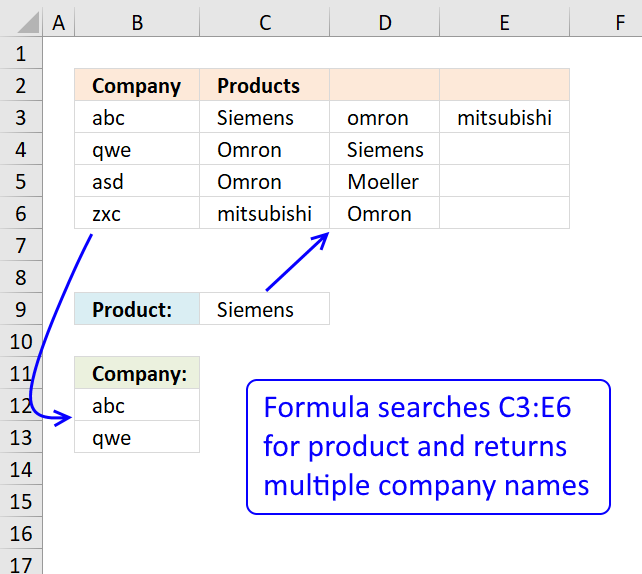
My database is as shown, where I have company abc sells siemens, omron and mitsubishi and company qwe sells omron n siemens.
Company Products
abc Siemens Omron Mitsubishi
qwe Omron Siemens
asd Omron Moeller
zxc Mitsubishi Omron
So right now I wanna key in the product name, lets say siemens, I hope it shows all the companies that sell siemens, in this case would be abc n qwe.
How is it possible? Using your formula can only works for first column, it will shows company abc only (first column), how to make it seach through the second column n show company qwe as well?
Answer:
This array formula looks up a value in a range (C3:E6) and returns multiple unique distinct values from a column (B3:B6). Cell C9 is the lookup value.
Excel 365 dynamic array formula in cell B12:
This array formula in cell B12 is for earlier Excel versions than Excel 365:
Watch a video where I explain how it works
How to create an array formula
- Double press with left mouse button on cell B12.
- Copy (Ctrl + c) and paste (Ctrl + v) above array formula to cell B12.
- Press and hold Ctrl + Shift simultaneously.
- Press Enter once.
- Release all keys.
How to copy array formula
- Select cell B12
- Copy (Ctrl + c)
- Select cell range B12:B14
- Paste ( Ctrl + v)
Explaining array formula in cell B12
Step 1 - Find matching values in array
($C$3:$E$6=$C$9)
returns {TRUE, FALSE, ... , FALSE}
Step 2 - Remove duplicate values in array
COUNTIF($B$11:B11, $B$3:$B$6)=0
returns {TRUE; TRUE; TRUE; TRUE}
Step 3 - Return row numbers
IF(($C$3:$E$6=$C$9)*(COUNTIF($B$11:B11, $B$3:$B$6)=0), ROW($C$3:$E$6)-MIN(ROW($C$3:$E$6))+1, "")
returns {1, "", "";"", 2, "";"", "", "";"", "", ""}
Step 4 - Find smallest row number
SMALL(IF(($C$3:$E$6=$C$9)*(COUNTIF($B$11:B11, $B$3:$B$6)=0), ROW($C$3:$E$6)-MIN(ROW($C$3:$E$6))+1, ""), 1)
becomes
SMALL({1, "", "";"", 2, "";"", "", "";"", "", ""}, 1)
and returns 1.
Step 5 - Return a value or reference of the cell at the intersection of a particular row and column
=INDEX($B$3:$B$6, SMALL(IF(($C$3:$E$6=$C$9)*(COUNTIF($B$11:B11, $B$3:$B$6)=0), ROW($C$3:$E$6)-MIN(ROW($C$3:$E$6))+1, ""), 1))
returns abc in cell B12.
2. VLOOKUP and return multiple values across columns

This section demonstrates a formula that lets you extract non-empty values across columns based on a condition. The image above shows the condition in cell B9 and the formula in cell range B10:B14.
The data set is in cell range A2:E7 and the lookup column is column A. The formula returns values from multiple rows if the corresponding value in the lookup column match, one value in each cell.
I geted the file lookup-vba3. I think I can use this to help me populate a calendar.I substituted dates for Pen, Paper, and Eraser. I then had locations substituted for $ values. Where I have a date of say, 11/27/12, I have 10 locations delivering that day.
Using the template as shown in the screenshot under "Return multiple values horizontally or vertically (VBA)".
I cannot expand past column "C" to return multiple values. I think it is in the array code but I cannot figure out how to return values past column C.
If you can help, greatly appreciated!
Thanks,
Jim
Answer:
Excel 365 dynamic array formula in cell B10:
Array formula in cell B10 for earlier Excel versions:
How to create an array formula
- Select cell B10.
- Press with left mouse button on in formula bar.
- Paste above array formula.
- Press and hold CTL + SHIFT simultaneously.
- Press Enter.
How to copy formula
- Select cell B10.
- Copy cell (Ctrl + c).
- Select cell range B11:B15.
- Paste (Ctrl + v).
The following array formula concatenates the returned values, the TEXTJOIN function is able to make the formula much smaller.
Array formula in cell B10:
Explaining array formula in cell B10
![]()
The INDEX function returns a value or a reference of the cell at the intersection of a particular column and row, in a given range.
INDEX($B$2:$E$7, row_num, column_num)
The first following three steps calculate the row_nums and the remaining steps calculate column_nums.
Step 1 - Find matching dates and non blanks
The equal sign is a logical operator. it lets you compare the value in cell B9 with cell range A2:A7, the logical expression returns TRUE if equal and FALSE if not.
$A$2:$A$7=$B$9
returns {TRUE; FALSE; ... ; TRUE}
The less than and greater than characters are also logical operators, they check if values in cell range B2:E7 are not blank.
$B$2:$E$7<>""
becomes
{"New York","Los Angeles",...,"San Francisco"}<>""
becomes
{TRUE, TRUE, ... , TRUE}
The parentheses allow you to manipulate the order of calculation which is really important in this step. The asterisk is a character that multiplies the two arrays, TRUE*TRUE = TRUE (1), TRUE*FALSE = FALSE (0) and FALSE * FALSE = FALSE (0). This means that AND logic is applied to the two arrays.
You can multiply arrays with different sizes as long as you follow certain rules, in this case, I am multiplying an array that has the same number of rows as the other array.
($A$2:$A$7=$B$9)*($B$2:$E$7<>"")
returns
{1, 1, ... , 0, 1}.
1 is the same as TRUE and 0 (zero) is FALSE. Excel converts the boolean values to their numerical equivalents when you perform arithmetic calculations between two or more arrays.
Step 2 - Return corresponding row numbers
IF(($A$2:$A$7=$B$9)*($B$2:$E$7<>""), MATCH(ROW($B$2:$E$7), ROW($B$2:$E$7)), "")
returns {1, 1, "", 1;... , 6}
Recommended articles
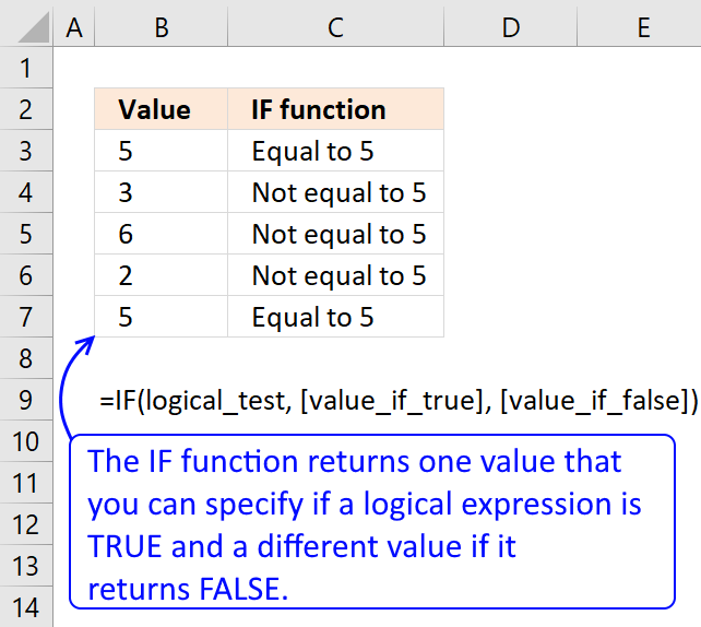
Checks if a logical expression is met. Returns a specific value if TRUE and another specific value if FALSE.
Step 3 - Return the k-th smallest value
SMALL(array, k)
SMALL(IF(($A$2:$A$7=$B$9)*($B$2:$E$7<>""), MATCH(ROW($B$2:$E$7), ROW($B$2:$E$7)), ""), ROW(A1))
becomes
SMALL({1, 1, "", 1;... , 6, "", 6}, 1)
and returns 1.
Recommended articles
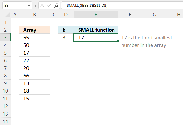
The SMALL function lets you extract a number in a cell range based on how small it is compared to the other numbers in the group.
Step 1 - Find matching dates and non blanks
($A$2:$A$7=$B$9)*($B$2:$E$7<>"")
returns {1, 1, 0... , 1}
Step 2 - Calculate both row numbers and column numbers
IF(($A$2:$A$7=$B$9)*($B$2:$E$7<>""), MATCH(ROW($B$2:$E$7), ROW($B$2:$E$7))+1/MATCH(COLUMN($B$2:$E$7), COLUMN($B$2:$E$7)), "")
returns {2,1.5,"",... ,6.25}
Step 3 - Return the k-th smallest value
SMALL(array, k)
SMALL(IF(($A$2:$A$7=$B$9)*($B$2:$E$7<>""), MATCH(ROW($B$2:$E$7), ROW($B$2:$E$7))+1/MATCH(COLUMN($B$2:$E$7), COLUMN($B$2:$E$7)), ""), ROW(A1))
returns 1.25.
Step 4 - Subtract row numbers
SMALL(IF(($A$2:$A$7=$B$9)*($B$2:$E$7<>""), MATCH(ROW($B$2:$E$7), ROW($B$2:$E$7))+1/MATCH(COLUMN($B$2:$E$7), COLUMN($B$2:$E$7)), ""), ROW(A1))-SMALL(IF(($A$2:$A$7=$B$9)*($B$2:$E$7<>""), MATCH(ROW($B$2:$E$7), ROW($B$2:$E$7)), ""), ROW(A1))
returns 0.25
Step 5 - Calculate column number
1/(SMALL(IF(($A$2:$A$7=$B$9)*($B$2:$E$7<>""), MATCH(ROW($B$2:$E$7), ROW($B$2:$E$7))+1/MATCH(COLUMN($B$2:$E$7), COLUMN($B$2:$E$7)), ""), ROW(A1))-SMALL(IF(($A$2:$A$7=$B$9)*($B$2:$E$7<>""), MATCH(ROW($B$2:$E$7), ROW($B$2:$E$7)), ""), ROW(A1)))
becomes
1/0.25 and returns column number 4.
Final calculation in cell B10
The INDEX function uses the row and column number to determine which value to return.
IFERROR(INDEX($B$2:$E$7, SMALL(IF(($A$2:$A$7=$B$9)*($B$2:$E$7<>""), MATCH(ROW($B$2:$E$7), ROW($B$2:$E$7)), ""), ROW(A1)), 1/(SMALL(IF(($A$2:$A$7=$B$9)*($B$2:$E$7<>""), MATCH(ROW($B$2:$E$7), ROW($B$2:$E$7))+1/MATCH(COLUMN($B$2:$E$7), COLUMN($B$2:$E$7)), ""), ROW(A1))-SMALL(IF(($A$2:$A$7=$B$9)*($B$2:$E$7<>""), MATCH(ROW($B$2:$E$7), ROW($B$2:$E$7)), ""), ROW(A1)))), "")
becomes
IFERROR(INDEX($B$2:$E$7, 1, 4), "")
becomes IFERROR("Chicago", "") and returns "Chicago" in cell B10.
If the INDEX function returns an error value the IFERROR function catches the error and returns a blank "".
Vlookup and return multiple values category

This post explains how to lookup a value and return multiple values. No array formula required.
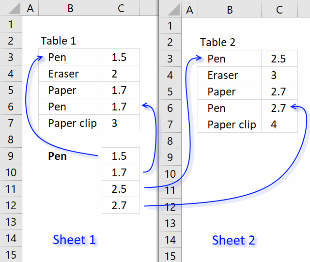
This article demonstrates an array formula that searches two tables on two different sheets and returns multiple results. Sheet1 contains […]
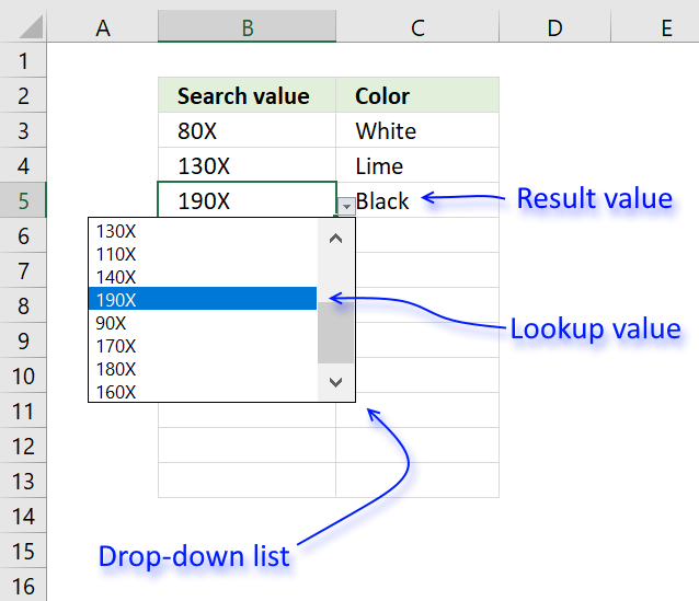
I will in this article demonstrate how to use a value from a drop-down list and use it to do […]
Excel categories
21 Responses to “Vlookup a cell range and return multiple values”
Leave a Reply
How to comment
How to add a formula to your comment
<code>Insert your formula here.</code>
Convert less than and larger than signs
Use html character entities instead of less than and larger than signs.
< becomes < and > becomes >
How to add VBA code to your comment
[vb 1="vbnet" language=","]
Put your VBA code here.
[/vb]
How to add a picture to your comment:
Upload picture to postimage.org or imgur
Paste image link to your comment.
Let's say that you only want to return the values in Column C (LA and Austin), how would the formula be written to accommodate this request? Also, what if you have numerical values in the cell and do not want blank cells to be included? How do you write the formula in that scenario? Thanks.
KO,
Array formula in cell B11:
Get the Excel *.xlsx file:
Lookup-and-return-multiple-values-from-a-range-excluding-blanks-KO.xlsx
What about the other way around? Lookup the location and return the dates?
Marco,
Your lookup location is in cell B16, array formula in cell B17:
=INDEX($A$2:$A$7, SMALL(IF($B$16=$B$2:$E$7, MATCH(ROW($B$2:$E$7), ROW($B$2:$E$7)), ""), ROW(A1)))
Thanks Oscar! It works that way but i noticed the cities don't repeat in different dates. What if they did? Is it possible to return multiple dates, i.e., what if Los Angeles was in two or more different dates?
I got it! But i still got a doubt. What if in between dates there were blanks and i don't want it to return blanks as well?
Got it was well! Thanks for the help!
=IFERROR(INDEX($B$2:$E$7, SMALL(IF(($A$2:$A$7=$B$9)*($B$2:$E$7""), MATCH(ROW($B$2:$E$7), ROW($B$2:$E$7)), ""), ROW(A1)), 1/(SMALL(IF(($A$2:$A$7=$B$9)*($B$2:$E$7""), MATCH(ROW($B$2:$E$7), ROW($B$2:$E$7))+1/MATCH(COLUMN($B$2:$E$7), COLUMN($B$2:$E$7)), ""), ROW(A1))-SMALL(IF(($A$2:$A$7=$B$9)*($B$2:$E$7""), MATCH(ROW($B$2:$E$7), ROW($B$2:$E$7)), ""), ROW(A1)))), "")
the formula okay but the size is problem, any possibility more efficient formulas?
Thanks
Rizky,
the formula okay but the size is problem, any possibility more efficient formulas?
I wish I knew a smaller formula but I don´t. Are you an excel 2003 user?
Nop Im just wonder another formula which more efficient, and my last question, could you tweak the formula so we can retrieve the value based on Column Header? Opposite from the case above which return values from Row Header as criteria....
Thanks
Can you please let me know what changes I need to make in this formula to have all the matching cities are populated in a single cell like
City1
City2
City3
Also I need to have a tooltip on the cell to show the description
his is the data table:
S/N RailCorp Ref Number Date In
77203 HRC mod program 10377 24/05/2011
77204 HRC mod program 10285 20/04/2011
77697 HRC mod program 10489 5/07/2011
77698 HRC mod program 10554 8/08/2011
77699 HRC mod program 10408 8/06/2011
77700 HRC mod program 10553 8/08/2011
77701 HRC mod program 10441 23/06/2011
77702 HRC mod program 10442 23/06/2011
77703 HRC mod program 10318 11/05/2011
77717 HRC mod program 10286 20/04/2011
77718 HRC mod program 10490 5/07/2011
79224 HRC mod program 10409 8/06/2011
79225 HRC mod program 10376 24/05/2011
79226 HRC mod program 10210 17/02/2011
79227 HRC mod program 10317 11/05/2011
I don't want to input the S/N in Table 2 manually. I need a formula for it as this is only part of the data that I need to categorise.
I need the S/N listed by the quarter they came in (Date In).
Yealy Quarter No Of Units S/N
Q1-2011 1
Q2-2011 10
Q3-2011 4
Q4-2011 0
Q1-2012 0
If someone can please help.
this is the result I am after but it should be done using formulas
Yealy Quarter No Of Units S/N
Q1-2011 1 79226
Q2-2011 10 77203, 77204, 77699, 77701, 77702, 77703, 77717, 79224, 79225, 79227
Q3-2011 4 77697, 77698, 77700, 77718
Q4-2011 0 NA
Q1-2012 0 NA
Thnaks in Advance
this is the data table:
S/N RailCorp Ref Number Date In
77203 HRC mod program 10377 24/05/2011
77204 HRC mod program 10285 20/04/2011
77697 HRC mod program 10489 5/07/2011
77698 HRC mod program 10554 8/08/2011
77699 HRC mod program 10408 8/06/2011
77700 HRC mod program 10553 8/08/2011
77701 HRC mod program 10441 23/06/2011
77702 HRC mod program 10442 23/06/2011
77703 HRC mod program 10318 11/05/2011
77717 HRC mod program 10286 20/04/2011
77718 HRC mod program 10490 5/07/2011
79224 HRC mod program 10409 8/06/2011
79225 HRC mod program 10376 24/05/2011
79226 HRC mod program 10210 17/02/2011
79227 HRC mod program 10317 11/05/2011
I don't want to input the S/N in Table 2 manually. I need a formula for it as this is only part of the data that I need to categorise.
I need the S/N listed by the quarter they came in (Date In).
Yealy Quarter No Of Units S/N
Q1-2011 1
Q2-2011 10
Q3-2011 4
Q4-2011 0
Q1-2012 0
If someone can please help.
this is the result I am after but it should be done using formulas
Yealy Quarter No Of Units S/N
Q1-2011 1 79226
Q2-2011 10 77203, 77204, 77699, 77701, 77702, 77703, 77717, 79224, 79225, 79227
Q3-2011 4 77697, 77698, 77700, 77718
Q4-2011 0 NA
Q1-2012 0 NA
Thnaks in Advance
Thanks a lot for this example. This is great!
I know this sounds a bit stupid, but..
The formula is printing cities going from E2 to B2 and then down a row.
What i need is to print them per column, going from B2 to B7, then C2 to C7, and so on.
Could you help??
I am banging my head on the wall :|
Hi Oscar,
I am using your formula here to pull some data from a Google Sheet that is linked to a Google Form. How can I tweak the formula to allow duplicates to be shown? The way I have it written right now, as long as the values that match the criteria are different, they are returned. If I have any duplicate values it only returns the first of those.
=INDEX('Form Responses 1'!$D$2:$D$1006, SMALL(IF(('Form Responses 1'!$C$2:$C$1006=$A$1)*(COUNTIF($G$13:G13,'Form Responses 1'!$D$2:$D$1006)=0), ROW('Form Responses 1'!$C$2:$C$1006)-MIN(ROW('Form Responses 1'!$C$2:$C$1006))+1, ""), 1))
My goal is to search the Form Responses for a name that's in a cell and return all of the values in a designated column that match the name. There will be a lot of duplicates and I need those in my data.
I appreciate any advice you can offer! Thank you for putting all of this information out there for folks like me!
Robert,
Based on the example in this article the following formula seems to work:
=INDEX($B$3:$B$6,SMALL(IF(($C$3:$E$6=$C$9),ROW($C$3:$E$6)-MIN(ROW($C$3:$E$6))+1,""),ROWS($A$1:A1)))
Get the Excel file:
Vlookup-a-cell-range-return-duplicates.xlsx
Hello,
I have a range of data with several columns.
on the first one (A:A) values are increasing from 1 to 1000.
I would like to get a copy, starting with no blank, of the values in A:A, B:B, C:C, etc... within a treshold of [5; 150] applied on A:A
What could be the function for that ?
Many thanks
Want to Extract Unique Distinct Value from 5 Different Cell
A J Entp 919825025403 919825025403 919825009822 919825025403 919825025403
A K Cera 919898363600 919898363600 919275017313
Aadi Ceramic 919898708413 919898708413
Aalishan 919825008579 919825008579
Aarti Cera 919157802760 919157802760
Aaryan Cera 919879832474 919879832474
Aatik ti 918347739973 918347739973 918347739973 918347739973 919879832474
Aavkar Trad 919909481398 919909481398
Absolute Floors 919817297172
=IFERROR(INDEX($B$2:$E$7, SMALL(IF(($A$2:$A$7=$B$9)*($B$2:$E$7""), MATCH(ROW($B$2:$E$7), ROW($B$2:$E$7)), ""), ROW(A1)), -1/(SMALL(IF(($A$2:$A$7=$B$9)*($B$2:$E$7""), MATCH(ROW($B$2:$E$7), ROW($B$2:$E$7))-1/MATCH(COLUMN($B$2:$E$7), COLUMN($B$2:$E$7)), ""), ROW(A1))-SMALL(IF(($A$2:$A$7=$B$9)*($B$2:$E$7""), MATCH(ROW($B$2:$E$7), ROW($B$2:$E$7)), ""), ROW(A1)))), "")
Need a formula to extract data based on text consider in Q column to get values of Column D & T in new sheet
if i have a running log of people calling off and i want to take that info and make it go into a calander that can be filtered by week ending dates what would be a formula for that?