Use a drop down list to search and return multiple values
Table of Contents
1. Use a drop down list to search and return multiple values
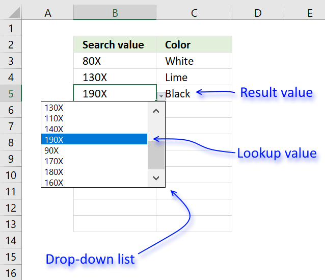
I will in this article demonstrate how to use a value from a drop-down list and use it to do a lookup in a dataset or preferably in an Excel defined Table. In other words, this will auto populate other cells when selecting values in a drop-down list.
I will also demonstrate how to create, edit and add values to a drop-down list. There are several kinds of drop-down lists in Excel. Data validation and Combo Boxes. They have their advantages and disadvantages and I will discuss them in this article.
Data validation drop-down list
The Data Validation drop-down list is easy to set up but it has its flaws, the purpose with data validation is to force the user to select one out of several predetermined values.
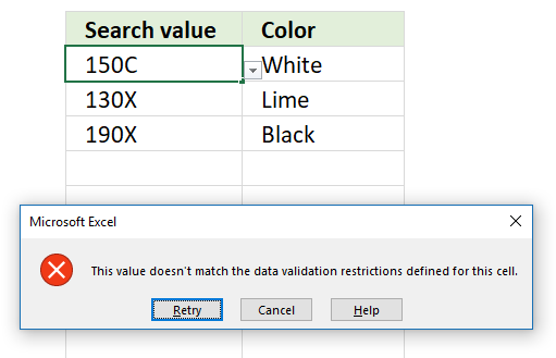
This can, however, be easily ignored by the user simply by pasting a value to the drop-down list.
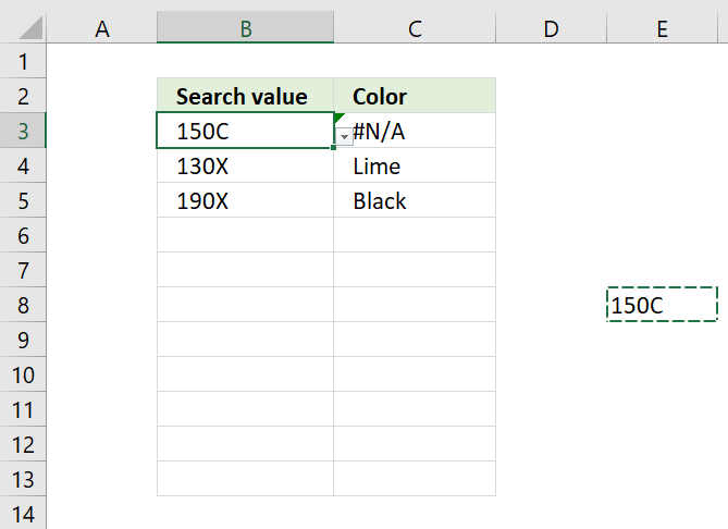
Another disadvantage is that the data validation drop-down list won't allow you to search for a value in the list, this can make it time-consuming and ineffective to use if it contains lots of values.
I recommend using a combo box if you want to be able to search a drop-down list. A combo box is also a drop-down list that you can easily create and manipulate.
Create a drop-down list
The data source is in this case an Excel defined Table which has its advantages. To be able to use it in a drop-down list a workaround is needed, the INDIRECT function makes it possible to reference the Table as a source.
- Select cell B3.
- Go to "Data" tab on the ribbon.
- Press with left mouse button on "Data Validation" button

- Select List
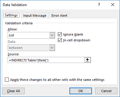
- Type =INDIRECT("Table1[Item]") in "Source:" window
- Press with left mouse button on OK
Formula that will auto populate a single cell
The first formula I will demonstrate is a simple INDEX - MATCH formula that will use the selected value in the drop-down list to search a dataset and return the adjacent value if a match is found.
Formula in cell C3:
The MATCH function returns the relative position of the drop-down list value in column Table1[Item] if found.
MATCH(Sheet1!$B3, Table1[Item],0) and returns 3. "80X" is found as the third value in the array.
The INDEX function returns the value in column Table1[Color] based on the relative position returned from the MATCH function.
INDEX(Table1[Color], MATCH(Sheet1!$B3, Table1[Item], 0)) returns "White in cell C3.
Formula that will auto populate several cells
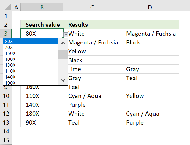
The following formula is more complicated, it returns multiple values distributed horizontally starting from column C.
Array formula in cell C3:
To enter an array formula, type the formula in cell C3 then press and hold CTRL + SHIFT simultaneously, now press Enter once. Release all keys.
The formula bar now shows the formula with a beginning and ending curly bracket telling you that you entered the formula successfully. Don't enter the curly brackets yourself.
Explaining formula in cell C3
Step 1 - Find cells that equal condition
Sheet2!$B3=Table1[Item] is a logical expression that returns boolean values, TRUE or FALSE.
Sheet2!$B3=Table1[Item] returns this array: {FALSE; FALSE; TRUE; ... ; FALSE}
Step 2 - Calculate row numbers of matching cells
The IF function has three arguments, the first one must be a logical expression. If the expression evaluates to TRUE then one thing happens (argument 2) and if FALSE another thing happens (argument 3).
The function replaces TRUE with the corresponding relative row number and FALSE with nothing "".
IF(Sheet2!$B3=Table1[Item], MATCH(ROW(Table1[Item]), ROW(Table1[Item])), "") returns {""; ""; 3; ... ; ""}.
Step 3 - Extract k-th smallest row number
To be able to return a new value in a cell each I use the SMALL function to filter column numbers from smallest to largest.
The COLUMNS function keeps track of the numbers based on an expanding cell reference. It will expand as the formula is copied to the cells below.
SMALL(IF(Sheet2!$B3=Table1[Item], MATCH(ROW(Table1[Item]), ROW(Table1[Item])), ""), COLUMNS($A$1:A1)) returns 3.
Step 4 - Return value from Excel defined Table
The INDEX function returns a value based on a cell reference and column/row numbers.
INDEX(Table1[Color], SMALL(IF(Sheet2!$B3=Table1[Item], MATCH(ROW(Table1[Item]), ROW(Table1[Item])), ""), COLUMNS($A$1:A1)))
returns "White" in cell C3.
Step 5 - Return blank if formula returns error
IFERROR(INDEX(Table1[Color], SMALL(IF(Sheet2!$B3=Table1[Item], MATCH(ROW(Table1[Item]), ROW(Table1[Item])), ""), COLUMNS($A$1:A1))), "")
The IFERROR handles all errors in a formula, it lets you specify a value to return if an error is found.
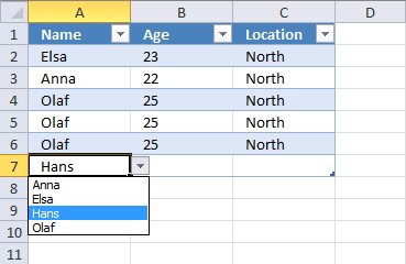
2. How to automatically add new items to a drop down list

A drop-down list in Excel prevents a user from entering an invalid value in a cell. Entering a value that is not in the drop-down list will not cause an error alert.
My worksheet allows you to type a new value and it is instantly included to the drop-down list. The drop-down list contains unique distinct values extracted from cells in the excel defined table.
The following animated picture shows what I am trying to explain.
The great thing about drop-down lists and excel defined tables is that you don't need to copy the drop-down list to new cells in the table. The Excel-defined table does that for you.
What's on this section
- Insert an Excel defined table
- Insert a new "helper" worksheet
- Create a new Excel Named Range
- Build a Drop-Down List
- How to disable Data Validation error alert
- Drop-Down List containing values sorted from A to Z
- Get Excel file
There is no VBA in this post. How is this done?
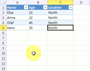
2.1. Insert an Excel defined table
Insert an Excel defined table or convert an existing range. You can use the shortcut keys CTRL + T or
- Go to tab "Insert" on the ribbon.
- Press with left mouse button on the "Table" button. A dialog box appears, see the image below.
- Make sure your data is selected and that the check box is enabled if you have table headers.
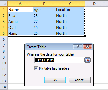
- Press with left mouse button on the OK button.

The table is now formatted differently,this makes it easy to identify Excel Tables on a worksheet.
2.2. Insert a new "helper" sheet
Insert a new sheet, it is going to be our "helper" sheet. I renamed it "Sheet2".
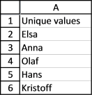
The formula in cell A2 extracts unique distinct values from Table1[Name].
Enter this array formula in cell A2:
Make sure you enter it as an array formula. If you don't know how follow these steps:
- Select cell A2
- Paste above formula to the formula bar
- Press and hold CTRL + SHIFT simultaneously
- Press Enter
- Release all keys.
If you did this right the formula now begins with a curly bracket { and ends with a curly bracket }. Don't enter these characters yourself.
Copy cell A2 and paste it to cells below as far as needed.
Update! Excel 365 dynamic array formula:
A dynamic array formula is not entered as an array formula. It works like a regular formula, press Enter only.
Read more about the UNIQUE function.
2.2.1 Explaining array formula in cell A2
Step 1 - Count cells based on a condition
The COUNTIF function counts cells that meet a condition.
COUNTIF('Sheet2'!$A$1:A1, Table1[Name])
returns {0; ... ; 0}.
Step 2 - Find relative position of the frist 0 (zero) in the array
The MATCH function returns the position of a given value in a cell range or array.
MATCH(lookup_value, lookup_array, [match_type])
MATCH(0,COUNTIF('Sheet2'!$A$1:A1, Table1[Name]), 0) returns 1.
Step 3 - Get value based on the relative position
The INDEX function returns a value from a cell range or array based on a row and column number.
INDEX(array, [row_num], [column_num])
INDEX(Table1[Name]&"", MATCH(0,COUNTIF('Sheet2'!$A$1:A1, Table1[Name]), 0))
returns "Elsa" in cell A2.
Step 4 - Return a blank if no value is found and an error is returned
IFERROR(INDEX(Table1[Name]&"", MATCH(0,COUNTIF('Sheet2'!$A$1:A1, Table1[Name]), 0)), "")
becomes
IFERROR("Elsa", "")
and returns "Elsa".
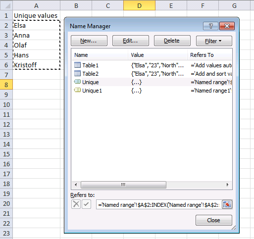
2.3. Create a new Excel Named Range
- Create a new named range by pressing CTRL + F3 or go to tab "Formulas" and press with left mouse button on the "Name Manager" button.
- Press with left mouse button on the "New..." button and use this formula:
='Sheet2'!$A$2:INDEX('Sheet2'!$A$2:$A$100, (1/IFERROR(1/SUM(IF('Sheet2'!$A$2:$A$100&"", 1, 0)), 1))) - Name it Unique. Remember to change the sheet reference if you use a different sheet name.
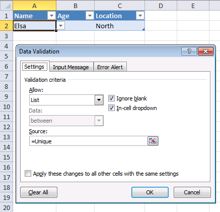
2.4. Build a Drop-Down List
- Go back to your excel defined table
- Create a drop-down list in one of the cells on the first row
- Go to tab "Data" on the ribbon
- Press with left mouse button on the "Data Validation" button on the ribbon
- Select List and type =Unique in the source field.
2.5. Disable data validation error alert
The "Error alert" ta in the data validation window allows you to remove the error alert that is shown after an invalid value is entered.
- Go to tab "Data" on the ribbon
- Press with left mouse button on the "Data validation" button
- Go to tab "Error alert"
- Disable "Show error alert after invalid data is entered"
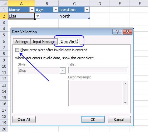
Disabling the error alert allows us to use the drop-down list if we want or type a new value in the cell.
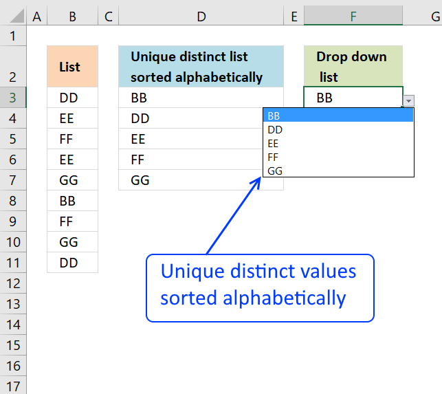
2.6. A sorted drop-down list from A to Z
The drop-down list in this sheet contains sorted text values, get the file below if you want to know how it is made.
If you want to learn more about array formulas join Advanced excel course.
Drop down lists category
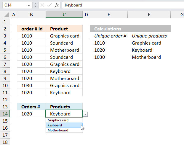
Table of Contents Create dependent drop down lists containing unique distinct values - Excel 365 Create dependent drop down lists […]
Question: How do I create a drop-down list with unique distinct alphabetically sorted values? Table of contents Introduction Sort values […]
Table of contents How to change cell formatting using a Drop Down list Highlight cells based on coordinates Highlight every […]
Vlookup and return multiple values category

This post explains how to lookup a value and return multiple values. No array formula required.
Excel categories
27 Responses to “Use a drop down list to search and return multiple values”
Leave a Reply
How to comment
How to add a formula to your comment
<code>Insert your formula here.</code>
Convert less than and larger than signs
Use html character entities instead of less than and larger than signs.
< becomes < and > becomes >
How to add VBA code to your comment
[vb 1="vbnet" language=","]
Put your VBA code here.
[/vb]
How to add a picture to your comment:
Upload picture to postimage.org or imgur
Paste image link to your comment.
thank you so much!!! Worked Perfectly
For some reason I am unable to 'ask a question' by the link, so, I thought i'll post it here since it is relevant to drop-down list.
In my workbook I have three worksheets; "Customer", "Vendor" and "Payment". In the Customer sheet I have a table, tblCustomer, where I add new customers. Similarly, in the Vendor sheet I have a table, tblVendor, where I add new vendors. In the Payment sheet I have a table, tblPayment, where i have three columns; Date, Amount and Name. Now, here is what I want to do; In the Name column of the tblPayment, I want to create a drop down list in each cell, which would contain all the names from tblCustomer[Name] and tblVendor[Name]. This way I can fill in the Date, Amount and then select one of all the names available in the drop down list of my Name cell. Is this possible without using VB code or any macro? If so, please help me out with this.
Rattan,
Read this post: Basic invoice template in excel
Pls the best way excel functions espeacially VLOOKUP / HLOOKUP etc to use in various way , columns, functions, multiple way.
rgds
abdussamed
Hi, I know this isn't array formula but maybe you can still help me. I have a spreadsheet that I use for 3 different companies.
What i would really like to do is have a drop down menu with the three company names: eg: Mcdonalds, Pizza Hut, Subway and then when i choose which company the spreadsheet will be for then all the contact information and logo will appear as a header on the top of the spread sheet. is this possible?
Hi one more question this array formula that you gave me earlier in the year, it's not working now.
I added another drop down box right beside the first one and i just want to take the exact same informaion so i dragged the formula to copy into the other cells and i just changed from B26 to B27 where the drop down menu is to look up.
Now it is not getting any of my informaion even though it's the exact same formula
Ainslie,
Can you provide both formulas? I am not sure whats wrong.
This is the original:
=IFERROR(INDEX(Panels!$C$2:$C$80, SMALL(IF($B$56=Panels!$A$2:$A$80, MATCH(ROW(Panels!$A$2:$A$80), ROW(Panels!$A$2:$A$80)), ""), ROW(A1))), "")
This is the one i'm trying to get to work. I need it to do the exact same thing in cells below where the original is used but both need to do the same thing just the drop down box where it has the information where to lookup is in a different location
=IFERROR(INDEX(Panels!$C$2:$C$80, SMALL(IF($B$57=Panels!$A$2:$A$80, MATCH(ROW(Panels!$A$2:$A$80), ROW(Panels!$A$2:$A$80)), ""), ROW(A1))), "")
Ainslie,
There seems to be nothing wrong with the formulas. Maybe the value ($B$57) in the drop down list doesnt exactly match some of the values in your list (Panels!$A$2:$A$80)?
nope, that's all the same, nothing has changed. it works in the other drop down box in B56 - the exact same values but not in B57
Aynsley Wall,
See this post: Use a drop down list to select company info in header (vba)
[...] me all the cars in my table that has the blue colour assigned to them. Similar to the code here Use a drop down list to search and return multiple values | Get Digital Help - Microsoft Excel resou... If i just had the one list box then fine, But I want many rows of list boxes that do the same [...]
Place the curser in cell A8 (your attached spreadsheet).
Press with right mouse button and select from the menu: "Pick_From Drop-Down List..." - works only for text.
Rarely used, even by the pro's.
//Ola.S
https://www.pcreview.co.uk/threads/pick-from-drop-down-list-gives-empty-or-erroneous-result.4026822/
Ola.S
I am not sure I understand.
Press with right mouse button and select from the menu: "Pick_From Drop-Down List..." - works only for text.
To be honest, I didn't know you could. That drop down list is not the same thing as a data validation rule - drop down list. Try it yourself, numbers work fine in my first example.
The drop down list is automatically copied to the next cell below when the table grows. Example, select the last cell in the table, cell C7 and press TAB key. A new row is inserted and cell A8 has a drop down list.
There are other ways to insert new table rows. Press with right mouse button on a cell and hover over "Insert". Press with left mouse button on "Insert Table rows above" or "Insert Table rows below"
Thank you for commenting.
Thanks' Oscar for sharing this trick.
I wonder what are the advantages of using tables?
mma173,
- Sort and filter
- Sum by adding a row for total
- By entering a formula in one cell in a table column, you can create a calculated column in which that formula is instantly applied to all other cells in that table column.
- Structured references
- Easy to reference a table or table column
- Formatting
- Easy to insert or delete table columns or rows
I got a question by email:
Is it possible to make a drop down list autocomplete if you have hundreds names instead of scrolling down into drop down list?
Yes, almost. It works only if the values in the drop down list are sorted.
Example
1. Type E in the cell
2. Press with left mouse button on the "Drop down list" arrow
3. You are now on letter E in the drop down list
4. Select a value
Helpful comments - Incidentally , if anyone have been needing to merge PDF or PNG files , I merged a tool here https://goo.gl/elSZt2.
Hey Oscar, thanks a lot for the method you outlined above! It helped me accomplish exactly what I'd set out to do. There is one issue I ran into using your instructions above, the formula you specify the reader's to use in step 2 of "Create a New Named Range" is:
='Sheet2'!$A$2:INDEX('Sheet2'!$A$2:$A$100,(1/IFERROR(1/SUM(IF('Sheet2'!$A$2:$A$100&"", 1, 0)), 1)))However, this formula would only list the value of A2 from "Sheet2" in my tables drop down list. After messing with it for a while I finally opened your example to find out where I went wrong & discovered that the formula you specified didn't match the formula you used in the example workbook! The formula in step 2 needs to be modified to include the less-than / greater-than (
) portion of the formula.Corrected formula should be:
='Sheet2'!$A$2:INDEX('Sheet2'!$A$2:$A$100,(1/IFERROR(1/SUM(IF('Sheet2'!$A$2:$A$100"",1,0)),1)))Thanks again Oscar!
-Jones
Hey Jones,
Thanks for the tip, I was having the same issue and couldn't figure out why.
Oscar, thank you for this review, it's saved me.
Ahh, it is automatically removing the less than / greater than symbols () in the code! :o/
MF Jones,
thank you for commenting.
Yes, wordpress removes html characters unfortunately.
Hey Oscar!
I am trying to make an automatically updating drop down menu. I am close to figuring it out. What I want to do is similar to what you have, except if a name gets deleted, I don't want it to go away on the list. Is this possible?
For instance, if the chart was one row and I typed in 3 name, all 3 names would show up on the named range, ultimately on the drop down list.
Michael,
I am trying to make an automatically updating drop down menu. I am close to figuring it out. What I want to do is similar to what you have, except if a name gets deleted, I don't want it to go away on the list. Is this possible?
Not with formulas, as far as I know.
For instance, if the chart was one row and I typed in 3 name, all 3 names would show up on the named range, ultimately on the drop down list.
There is no chart in this article?
Hello Oscar, great post and very helpful. If starting a new workbook, with an existing list of 20-30 items of data i want available for the drop down, but with the table only having 3-4 of these so far, can the other items be included in the drop-down list? At the moment, they only show if included in the table.
Thanks again.
Oscar, Thanks for the method to automatically add and sort drop-down list items. I've been trying to resolve one issue, which I can't seem to figure out (ref. your Excel spreadsheet). What I’ve found is that if there’s a name in the first row of the "Name" column of the "Table2" ("Add and sort values" sheet), everything works as expected. That's even true if there are rows below the first row of the "Name" column of the "Table2" that do not have a name in them, i.e., blank cells between cells with names. However, the issue I've come across is that if there's not a name in the first row of the "Name" column of the "Table2", any names in any of the rows below the first row are ignored. I can't seem to resolve why the array formula in the column "A" cells on the "Named range1" sheet require a name in the first row of "Table2". I was hoping you could provide some insight as to why this is happening and a possible fix to allow the first row to be blank and have non-blank rows below. I've provided a photo of with and without a name on the first row--see link embedded.
https://imgur.com/nNvHvbW
Can this be done in Google Sheets?