Create numbers based on numerical ranges
Table of Contents
1. Create numbers based on numerical ranges - Excel 365
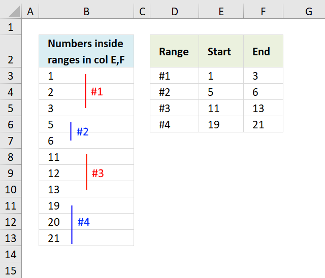
The image above demonstrates a formula in cell B3 that lists numbers from 1 to 21 only if they meet the numerical ranges specified in cell range E3:F6.
The first numerical range is 1 to 3, the second is 5 to 6, the third is 11 to 13, and the last one is 19 to 21. The numbers that meet these criteria are listed in cell B3 and cells below as far as needed. They are 1, 2, 3, 5, 6, 11, 12, 13, 19, 20, and 21. The numbers that don't meet the criteria in cell range E3:F6 are 4, 7, 8, 9, 10, 14, 15, 16, 17, and 18.
Excel 365 dynamic array formula in cell B3:
1.2 Explaining the formula
Step 1 - Build an array containing numbers from 1 to 21
The ROW function calculates the row number of a cell reference.
Function syntax: ROW(reference)
ROW(A1:A21)
returns
{1; 2; ... ; 21}
Step 2 - Check numbers that meet criteria
The COUNTIFS function calculates the number of cells across multiple ranges that equals all given conditions.
Function syntax: COUNTIFS(criteria_range1, criteria1, [criteria_range2, criteria2]…)
COUNTIFS($E$3:$E$6, "<="&ROW(A1:A21),$F$3:$F$6, ">="&ROW(A1:A21))
becomes
COUNTIFS({1;5;11;19}, "<="&{1; 2; ... ; 21},{3;6;13;21}, ">="&{1; 2; ... ; 21})
and returns
{1; 1; 1; 0; 1; 1; 0; 0; 0; 0; 1; 1; 1; 0; 0; 0; 0; 0; 1; 1; 1}
Step 3 - Filter numbers based on array
The FILTER function extracts values/rows based on a condition or criteria.
Function syntax: FILTER(array, include, [if_empty])
FILTER(ROW(A1:A21),COUNTIFS($E$3:$E$6, "<="&ROW(A1:A21),$F$3:$F$6, ">="&ROW(A1:A21)))
returns {1; 2; 3; 5; 6; 11; 12; 13; 19; 20; 21}
Step 4 - Shorten formula
The LET function lets you name intermediate calculation results which can shorten formulas considerably and improve performance.
Function syntax: LET(name1, name_value1, calculation_or_name2, [name_value2, calculation_or_name3...])
ROW(A1:A21) is repeated three times in the formula.
FILTER(ROW(A1:A21),COUNTIFS($E$3:$E$6, "<="&ROW(A1:A21),$F$3:$F$6, ">="&ROW(A1:A21)))
x - ROW(A1:A21)
LET(x,ROW(A1:A21),FILTER(x,COUNTIFS($E$3:$E$6, "<="&x,$F$3:$F$6, ">="&x)))
2. Create numbers based on numerical ranges - earlier Excel versions
The image above shows an array formula in cell B3 that calculates numbers based on the numerical ranges in cell range E3:F6.
Array formula in B3:
To enter an array formula, type the formula in a cell then press and hold CTRL + SHIFT simultaneously, now press Enter once. Release all keys.
The formula bar now shows the formula with a beginning and ending curly bracket telling you that you entered the formula successfully. Don't enter the curly brackets yourself.
Explaining formula in cell B3
Step 1 - Create a sequence
The ROW function returns a row number based on a cell reference, if the cell reference has multiple rows then the row function returns an array of numbers.
ROW($1:$21)
returns
{1; 2; 3; 4; 5; 6; 7; 8; 9; 10; 11; 12; 13; 14; 15; 16; 17; 18; 19; 20; 21}
Step 2 - Check if number is in sequence
The COUNTIFS function checks if a number is larger or equal to the start value and smaller or equal to the end value. If both conditions are met the COUNTIFS function returns 1.
COUNTIFS($E$3:$E$6, "<="&ROW($1:$21),$F$3:$F$6, ">="&ROW($1:$21))
returns {1; 1; 1; 0; 1; 1; 0; 0; 0; 0; 1; 1; 1; 0; 0; 0; 0; 0; 1; 1; 1}
Tip! Use an Excel defined Table to create dynamic cell references that you don't have to adjust if more ranges are added or deleted.
Step 3 - Return number if in range
The IF function has three arguments, the first one must be a logical expression. If the expression evaluates to TRUE then one thing happens (argument 2) and if FALSE another thing happens (argument 3).
IF(COUNTIFS($E$3:$E$6, "<="&ROW($1:$21),$F$3:$F$6, ">="&ROW($1:$21)), ROW($1:$21))
returns {1; 2; 3; FALSE; 5; 6; FALSE; FALSE; FALSE; FALSE; 11; 12; 13; FALSE; FALSE; FALSE; FALSE; FALSE; 19; 20; 21}.
Step 4 - Extract k-th smallest number
The ROWS function keeps track of the numbers based on an expanding cell reference. It will expand as the formula is copied to the cells below.
SMALL(IF(COUNTIFS($E$3:$E$6, "<="&ROW($1:$21),$F$3:$F$6, ">="&ROW($1:$21)), ROW($1:$21)), ROWS($A$1:A1))
becomes SMALL({1; 2; ... ; 21}, 1) and returns 1 in cell B3.
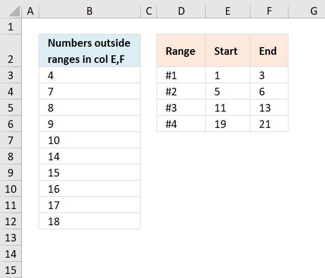
The array formula in cell B3 lists numbers not in ranges specified in cell range E3:F6.
Array formula in B3:
More than 1300 Excel formulas
Excel categories
One Response to “Create numbers based on numerical ranges”
Leave a Reply
How to comment
How to add a formula to your comment
<code>Insert your formula here.</code>
Convert less than and larger than signs
Use html character entities instead of less than and larger than signs.
< becomes < and > becomes >
How to add VBA code to your comment
[vb 1="vbnet" language=","]
Put your VBA code here.
[/vb]
How to add a picture to your comment:
Upload picture to postimage.org or imgur
Paste image link to your comment.
Hello,
Thanks for this helpful information on excel formulas.
I need help with counting the number of cells that fall outside of two numbers, so I need to get the count of numbers that are less than -0.1 and greater than 0.1. I have been searching online for a long time, but everyone talks about counting the values that fall with in two numbers, but no discussion on how to count the numbers that are outside two numbers. I have tried COUNTIFS, but it won't work, it will only work to count numbers with in two numbers.
Any help is appreciated. Thank you!