How to use the ROW function

What is the ROW function?

The ROW function calculates the row number of a cell reference.

1. Syntax

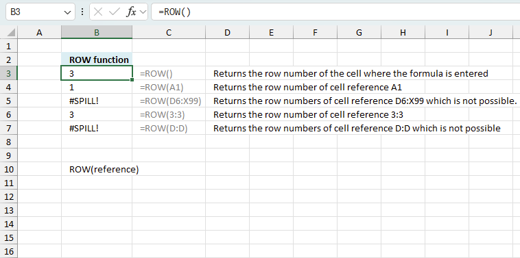
ROW(reference)

Back to top

2. Arguments

reference

Optional. A reference to a cell you want to know the row number of.

The ROW function is one of my most used Excel functions, that you probably already know if you have been browsing around my web site.

The first example demonstrates basic usage. Example 2 and 3 are more advanced and requires some knowledge about MATCH and INDEX function.

Back to top

3. Example 1 - Cell references

You can enter a reference to a single cell or a cell range in the ROW function. Note that it will return an array of numbers if you enter a reference to a cell range, as long as you enter it as an array formula.

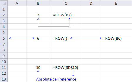
Formula in cell B2:

B2 is a relative cell reference meaning it changes when you copy the cell and pastes it to another cell.

ROW(B2)

returns 2.

Formula in cell B6:

This example shows that you can omit the argument, the formula will default to the cell where the formula is entered.

The formula is entered in cell B6 in the example above, so it returns 6.

Formula in cell B11:

$D$10 is an absolute cell reference meaning it won't change if you copy the cell and paste to other cells. Absolute and relative references in Excel

returns 10.

The following example is not demonstrated in the image above. Type this formula in any cell:

To enter the formula as an array formula, follow these steps: Press and hold CTRL + SHIFT simultaneously, then press Enter. Release all keys.

The formula is now surrounded by curly brackets, like this: {=ROW(A2:A5)}. Don't enter these characters yourself, they appear automatically.

The cell will now only show the first value in the array which is 2, you must enter the array formula in a cell range equal of size as there are values in the array to be able to see them all.

Update - Dynamic arrays

Office 365 subscribers can now take advantage of dynamic arrays. They behave differently than regular array formulas, simply enter them as a regular formula and Excel will automatically extend the formula to cells below so you can see all values.

This behavior is called spilling, see image above. The cell range containing spilled values have a blue border, it will disappear as soon as you press with left mouse button on outside the cell range.

Microsoft recommends that you use dynamic arrays instead of regular array formulas, however, they are still working and compatible with older Excel versions.

Back to top

4. Create an array of sequential numbers

The image above demonstrates a formula that creates an array of sequential numbers from 1 to 4. This can be used to number any cell range in order to get the appropriate values/rows.

Here are a few examples: Extract all rows from a range that meet the criteria in one column | 5 easy ways to VLOOKUP and return multiple values | INDEX MATCH - partial match multiple columns

Excel 365 subscribers can use the SEQUENCE function which offers more granular control. Most Excel 365 functions don't need the SEQUENCE function to number values/rows. For example, the FILTER function keeps track of values by itself.

Array formula in cell B2:

4.1 How to enter an array formula

1. Select cell range B2:B5 with your mouse.
2. Type: =ROW(A1:A4)
3. Press and hold CTRL + SHIFT keys simultaneously.
4. Press Enter once.
5. Release all keys.

The formula in the formula bar has a leading and ending curly bracket, they appear automatically when you follow all 5 steps above.

Don't enter these characters yourself.

Back to top

5. Example 2 - Duplicate columns in an array

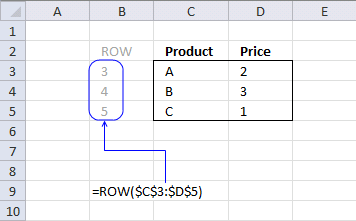
This example demonstrates that if you provide a cell reference pointing to a cell range containing multiple columns the formula will still only return a single column of row numbers.

returns this array {3; 4; 5}.

The semicolon is a separating character telling you that the values are on a row each. A comma is used to separate values distributed across columns.

Now you might wonder why the array formula doesn´t return {3, 3; 4, 4; 5, 5}. There are six cells in the cell range, how come only three values are returned?

The answer is that there is no need for multiple duplicate columns in the array. Excel simplifies the array down to a single column.

But when used with multiple cell ranges in more complicated array formulas, make sure the number of rows matches.
See this example: Unique distinct values from a cell range

Back to top

6. Example 3 - Number rows in any cell range

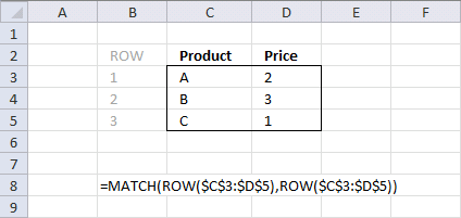
The INDEX function returns a value of the cell at the intersection of a particular row and column, in a given range. To be able to work with multiple values from an arbitrary cell range using the INDEX function we must number each row.

That is exactly what we did in the previous example but the first row in a given range has to be 1 and the second 2 and so on. Why? The INDEX function needs properly numbered cell ranges. This is where the ROW and MATCH function comes in.

The beauty with this formula is that it returns row numbers from any cell range no matter size or location.

Array formula in cell range B3:B5:

becomes =MATCH({3; 4; 5}, {3; 4; 5}) and returns {1; 2; 3}. This array has the same number of values as there are rows in cell range C3:D5.

Remember, enter the formula as an array formula.

So what can you do with row numbered cell ranges?

• How to return multiple values using vlookup
  
• Match two criteria and return multiple rows in excel

The MATCH function can also be used to find the relative position of a value in a cell range. See these posts:

• How to extract unique distinct values from a column
  
• Repeat values
• Fetch data from another table
• Shift Schedule

Back to top

7. How to number rows?

The image above demonstrates how to number records in a data set, however, this method is not great and I will show you why.

Here are the steps:

1. Select cell B3.
2. Type: =ROW(A1)
3. Press Enter.
4. Copy cell B3.
5. Paste to cells below as far as needed.

Why not use this formula? The formula will break if you insert more rows above, the cell reference is relative meaning it will change. The same thing will happen with an absolute formula.

I recommend you use the ROWS function with an expanding cell reference.

Formula in cell B3:

Copy cell B3 and paste to cells below, this will adjust the expanding cell reference accordingly. This will not break if you insert more rows.

Back to top

8. Function not working

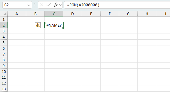
The ROW function returns #NAME? error

•  if you misspell the function name
• specify an invalid cell reference

8.1 Troubleshooting the error value

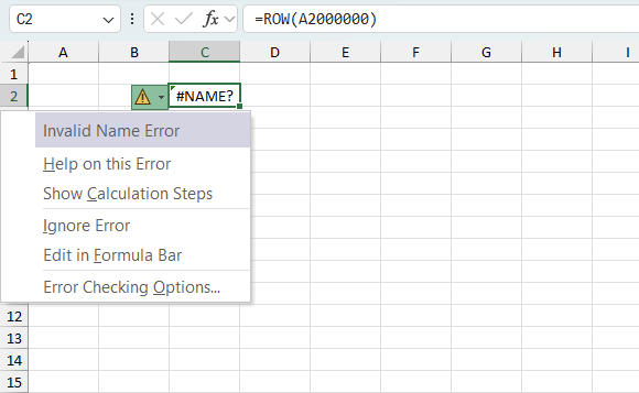
When you encounter an error value in a cell a warning symbol appears, displayed in the image above. Press with mouse on it to see a pop-up menu that lets you get more information about the error.

1. The first line describes the error if you press with left mouse button on it.
2. The second line opens a pane that explains the error in greater detail.
3. The third line takes you to the "Evaluate Formula" tool, a dialog box appears allowing you to examine the formula in greater detail.
4. This line lets you ignore the error value meaning the warning icon disappears, however, the error is still in the cell.
5. The fifth line lets you edit the formula in the Formula bar.
6. The sixth line opens the Excel settings so you can adjust the Error Checking Options.

Here are a few of the most common Excel errors you may encounter.

#NULL error - This error occurs most often if you by mistake use a space character in a formula where it shouldn't be. Excel interprets a space character as an intersection operator. If the ranges don't intersect an #NULL error is returned. The #NULL! error occurs when a formula attempts to calculate the intersection of two ranges that do not actually intersect. This can happen when the wrong range operator is used in the formula, or when the intersection operator (represented by a space character) is used between two ranges that do not overlap. To fix this error double check that the ranges referenced in the formula that use the intersection operator actually have cells in common.

#SPILL error - The #SPILL! error occurs only in version Excel 365 and is caused by a dynamic array being to large, meaning there are cells below and/or to the right that are not empty. This prevents the dynamic array formula expanding into new empty cells.

#DIV/0 error - This error happens if you try to divide a number by 0 (zero) or a value that equates to zero which is not possible mathematically.

#VALUE error - The #VALUE error occurs when a formula has a value that is of the wrong data type. Such as text where a number is expected or when dates are evaluated as text.

#REF error - The #REF error happens when a cell reference is invalid. This can happen if a cell is deleted that is referenced by a formula.

#NAME error - The #NAME error happens if you misspelled a function or a named range.

#NUM error - The #NUM error shows up when you try to use invalid numeric values in formulas, like square root of a negative number.

#N/A error - The #N/A error happens when a value is not available for a formula or found in a given cell range, for example in the VLOOKUP or MATCH functions.

#GETTING_DATA error - The #GETTING_DATA error shows while external sources are loading, this can indicate a delay in fetching the data or that the external source is unavailable right now.

8.2 The formula returns an unexpected value

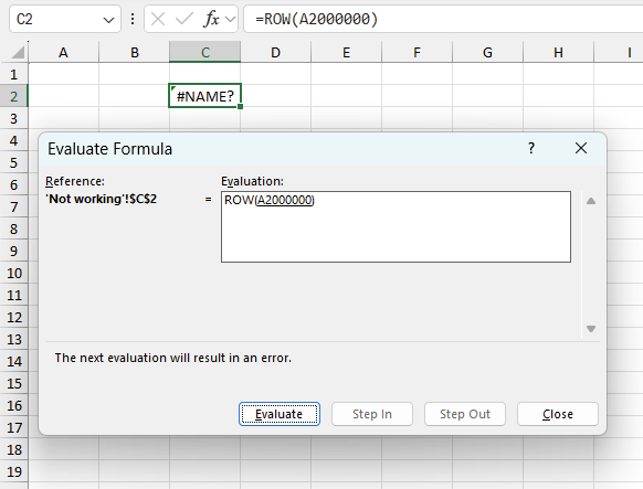
To understand why a formula returns an unexpected value we need to examine the calculations steps in detail. Luckily, Excel has a tool that is really handy in these situations. Here is how to troubleshoot a formula:

1. Select the cell containing the formula you want to examine in detail.
2. Go to tab “Formulas” on the ribbon.
3. Press with left mouse button on "Evaluate Formula" button. A dialog box appears.
   The formula appears in a white field inside the dialog box. Underlined expressions are calculations being processed in the next step. The italicized expression is the most recent result. The buttons at the bottom of the dialog box allows you to evaluate the formula in smaller calculations which you control.
4. Press with left mouse button on the "Evaluate" button located at the bottom of the dialog box to process the underlined expression.
5. Repeat pressing the "Evaluate" button until you have seen all calculations step by step. This allows you to examine the formula in greater detail and hopefully find the culprit.
6. Press "Close" button to dismiss the dialog box.

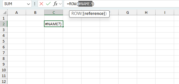
There is also another way to debug formulas using the function key F9. F9 is especially useful if you have a feeling that a specific part of the formula is the issue, this makes it faster than the "Evaluate Formula" tool since you don't need to go through all calculations to find the issue..

1. Enter Edit mode: Double-press with left mouse button on the cell or press F2 to enter Edit mode for the formula.
2. Select part of the formula: Highlight the specific part of the formula you want to evaluate. You can select and evaluate any part of the formula that could work as a standalone formula.
3. Press F9: This will calculate and display the result of just that selected portion.
4. Evaluate step-by-step: You can select and evaluate different parts of the formula to see intermediate results.
5. Check for errors: This allows you to pinpoint which part of a complex formula may be causing an error.

The image above shows cell reference A2000000 converted to hard-coded value using the F9 key. The ROW function requires valid cell references which is not the case in this example. We have found what is wrong with the formula.

Tips!

• View actual values: Selecting a cell reference and pressing F9 will show the actual values in those cells.
• Exit safely: Press Esc to exit Edit mode without changing the formula. Don't press Enter, as that would replace the formula part with the calculated value.
• Full recalculation: Pressing F9 outside of Edit mode will recalculate all formulas in the workbook.

Remember to be careful not to accidentally overwrite parts of your formula when using F9. Always exit with Esc rather than Enter to preserve the original formula. However, if you make a mistake overwriting the formula it is not the end of the world. You can “undo” the action by pressing keyboard shortcut keys CTRL + z or pressing the “Undo” button

8.3 Other errors

Floating-point arithmetic may give inaccurate results in Excel - Article

Floating-point errors are usually very small, often beyond the 15th decimal place, and in most cases don't affect calculations significantly.

Back to top

'ROW' function examples

Functions in 'Lookup and reference' category

The ROW function function is one of 25 functions in the 'Lookup and reference' category.

Excel function categories

Excel categories

Comments (1)