How to use the COUNTIFS function
What is the COUNTIFS function?
The COUNTIFS function calculates the number of cells across multiple ranges that equals all given conditions.
It allows you to use up to 254 arguments or 127 criteria pairs.
What's on this page
- Syntax
- Arguments
- Example 1
- Example 2 - Partial match using wildcard characters
- Example 3 - using two conditions
- Example 4 - Logical operators
- Example 5 - Count duplicate records
- Example 6 - return an array identifying records based on multiple conditions
- Example 7 - OR logic
- Example 8 - how to use dates
- Example 9 - after a date
- Example 10 - before a date
- How to make the function work with a dynamic range
- How to count entries in Excel by date and an additional condition
- Function not working
- Get Excel *.xlsx file
1. Syntax
COUNTIFS(criteria_range1, criteria1, [criteria_range2, criteria2]…)
2. Arguments
| criteria_range1 | Required. The cell range you want to count the cells meeting a condition. |
| criteria1 | Required. The condition that you want to count. |
| [criteria_range2] | Optional. Additional ranges, up to 127 pairs. |
| [criteria2] | Optional. Additional ranges, up to 127 pairs. |
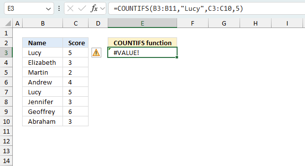
3. Example 1
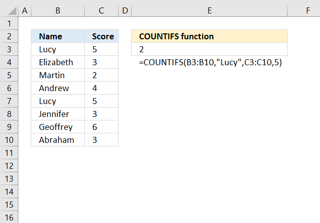
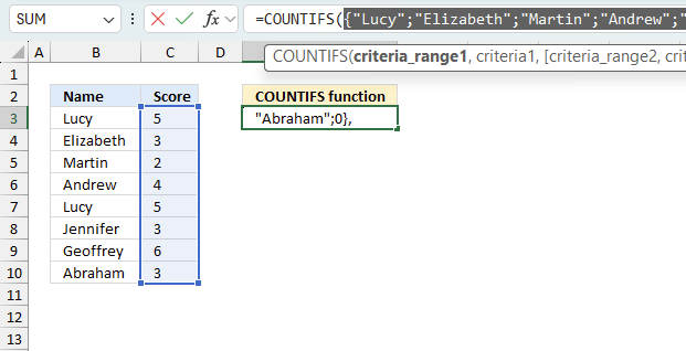
The COUNTIFS function counts the number of rows that matches one or more conditions. The image above shows the following data table in cell range B3:C10:
| Name | Score |
| Lucy | 5 |
| Elizabeth | 3 |
| Martin | 2 |
| Andrew | 4 |
| Lucy | 5 |
| Jennifer | 3 |
| Geoffrey | 6 |
| Abraham | 3 |
Formula in cell E3:
Lucy and 5 are found twice, in rows 3 and 7. The COUNTIFS function returns 2 in cell E3 which represents the number of times both conditions match on a single row. All conditions must be met on the same row.
The COUNTIFS function lets you use many condition pairs, this example shows only two. A pair meaning a condition and the corresponding cell range you want to use.
This function is excellent for counting unique, unique distinct or duplicate rows etc. You can do some seriously complicated calculations with this function.
4. Example 2 - Partial match using wildcard characters

The optional wildcard characters make the COUNTIFS function even more powerful, these characters are * asterisk and question marks ? The question mark ? matches a single character while the * asterisk matches any sequence of characters even 0 (zero) characters.
The image above shows this data table in cell range B3:C10:
| Name | Country |
| Lucy | Canada |
| Elizabeth | US |
| Martin | France |
| Andrew | Spain |
| Steve | Italy |
| Jennifer | Canada |
| Geoffrey | Italy |
| Abraham | France |
Cell E3 contains the following condition: *n*, cell F3 contains the second condition which is *an* The asterisks allow you to match any characters from zero to any number.
For example, *n* matches cell B5 because the value ends with a "n", cell C5 matches *an* because it is found in this value "France", in other words, the asterisk allows you to perform a partial match.
Formula in cell E6:
The next match is found in cell B8, "Jennifer" contains the character "n" and cell C8 which is "Canada" contains "an". Remember that both conditions must be matched for the COUNTIFS function to add the row to the total count.
There are plenty more matches in B3:C10, however, rows 5 and 8 are the only ones that matches both conditions.
4.1 Explaining formula
The Evaluate Formula tool is located on the Formulas tab in the Ribbon. It is a useful feature that allows you to step through and evaluate complex formulas to understand how the calculation is being performed and identify any errors or issues. The following steps shows these detailed evaluations for the formula above.
Step 1 - Populate arguments
COUNTIFS(criteria_range1, criteria1, [criteria_range2, criteria2]…)
criteria_range1 - B3:B10
criteria1 - E3
criteria_range2 - C3:C10
criteria2 - F3
COUNTIFS(B3:B10, E3, C3:C10, F3)
Step 2 - Evaluate COUNTIFS function
COUNTIFS(B3:B10, E3, C3:C10, F3)
becomes
COUNTIFS({"Lucy"; "Elizabeth"; "Martin"; "Andrew"; "Steve"; "Jennifer"; "Geoffrey"; "Abraham"}, "*n*", {"Canada"; "US"; "France"; "Spain"; "Italy"; "Canada"; "Italy"; "France"}, "*an*")
The asterisk matches 0 (zero) to any number of characters, and a leading and trailing asterisk "*n*" matches any value that contains the character n in cells B3:B10. "Martin", "Andrew", "Jennifer" contains a "n"
"*an*" matches any country in cells C3:C10 that contains "an", they are found in rows 3, 5, 8, and 10. The COUNTIFS function counts a row if both conditions are met.
COUNTIFS({"Lucy"; "Elizabeth"; "Martin"; "Andrew"; "Steve"; "Jennifer"; "Geoffrey"; "Abraham"}, "*n*", {"Canada"; "US"; "France"; "Spain"; "Italy"; "Canada"; "Italy"; "France"}, "*an*")
returns
2.
5. Example 3 - using two conditions
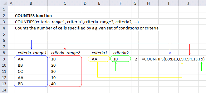
This example demonstrates the COUNTIFS function with two conditions applied to two separate columns. The COUNTIFS function counts a record when both conditions are met on the same row.
This formula checks if text string "AA" is found in cell range B9:B13 and if 10 is found in cell range C9:c13. Row 9 and 12 contain both conditions and 2 are returned to cell G9.
COUNTIFS(B9:B13,E9,C9:C13,F9)
becomes
COUNTIFS({"AA";"BB";"CC";"AA";"BB"},"AA",{10;20;30;10;40},10)
and returns 2 in cell G9.
The calculation above shows two arrays and ou can tell that by the curly brackets {}.
The values in those arrays are separated by a semicolon meaning the values are on a row each.
Here is a post where I use this technique: Highlight duplicate rows
6. Example 4 - Logical operators
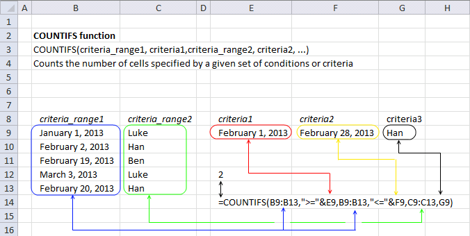
The following formula counts how many times text string "Han" equals a cell value in cell range C9:C13, it also checks if dates in cell range B9:B13 are larger than or equal to February 1st, 2013 and smaller than or equal to February 28, 2013.
Three conditions in total are applied to two cell ranges, this also demonstrates that you can use logical operators with conditions. Make sure you use double quotes enclosing the logical operators and an ampersand to concatenate the values with the logical operators.
Here is a list of all logical operators you can use and their combinations.
- = equal to
- < less than
- > larger than
- <= less than or equal to
- >=larger than or equal to
- <> not equal to
COUNTIFS(B9:B13, ">="&E9, B9:B13, "<="&F9, C9:C13, G9)
becomes
COUNTIFS({41275; 41307; 41324; 41336; 41325}, ">="&41306, {41275; 41307; 41324; 41336; 41325}, "<="&41333, {"Luke"; "Han"; "Ben"; "Luke"; "Han"}, "Han")
and returns 2 in cell E12. Row 9 and 13 have the word "Han" and are in the month of February 2013.
Here is a post where I use comparison operators: Filter overlapping date ranges
7. Example 5 - Count duplicate records
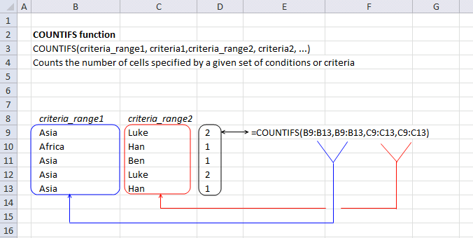
The following array formula counts each cell value in each row and returns an array of values.
I demonstrated in example 1 and 2 above how to use a single condition in each criteria argument, the formula above demonstrates what happens if you use multiple conditions.
Note, you will receive an error if you don't use the same number of conditions in each criteria argument.
COUNTIFS(B9:B13, B9:B13, C9:C13, C9:C13)
becomes
COUNTIFS({"Asia"; "Africa"; "Asia"; "Asia"; "Asia"},{"Asia"; "Africa"; "Asia"; "Asia"; "Asia"},{"Luke"; "Han"; "Ben"; "Luke"; "Han"},{"Luke"; "Han"; "Ben"; "Luke"; "Han"})
and returns this array {2; 1; 1; 2; 1} in cell range D9:D13. This array is interesting because it identifies how many times each record occurs in the data set.
Here are two posts where I use this technique:
8. Example 6 - return an array identifying records based on multiple conditions
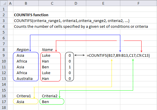
In this example, I am using a single cell value as a criteria_range argument and a cell range as criteria argument. This may seem confusing but it is definitely possible and sometimes very useful.
The image above shows this data table in cell range B8:C13:
| criteria_range1 | criteria_range2 |
| Asia | Luke |
| Africa | Han |
| Asia | Ben |
| Asia | Luke |
| Asia | Han |
The first condition is specified in cell B17 and the second condition in cell C17. We are using one condition in the criteria1 argument and a cell reference to one cell in the criteria_range argument. This is true for the second condition as well.
Array formula in cell D9:D13
This setup makes the COUNTIFS function return an array as large as the source data range. The output returns 1 if the row matches the criteria and 0 (zero) if not.
For example, the output from the formula is displayed in cell D9 and cells below. They correspond to the source data range specified in B8:C13 meaning that 1 identifies that particular row as a match. The example above returns 1 only for row 11, in other words, row 11 is the only record that matches both conditions.
8.1 How to enter an array formula
Excel 365 users can skip these steps, press Enter to enter the formula like a regular formula.
- Select cells D9:D13.
- Type the formula above: =COUNTIFS(B17,B9:B13,C17,C9:C13)
- Press and hold CTRL + SHIFT simultaneously.
- Press Enter once.
- Release all keys.
The formula is now enclosed with curly brackets like this: {=COUNTIFS(B17,B9:B13,C17,C9:C13)}
Don't enter these characters yourself, they appear automatically if you followed the steps above.
8.2 Explaining the formula
The Evaluate Formula tool is located on the Formulas tab in the Ribbon. It is a useful feature that allows you to step through and evaluate complex formulas to understand how the calculation is being performed and identify any errors or issues. The following steps shows these detailed evaluations for the formula above.
COUNTIFS(B17, B9:B13, C17, C9:C13)
becomes
COUNTIFS("Asia", {"Asia"; "Africa"; "Asia"; "Africa"; "Australia"}, "Ben", {"Luke"; "Han"; "Ben"; "Luke"; "Han"})
and returns
{0; 0; 1; 0; 0}
in cell range D9:D13.
Row three meets all conditions, 1 is in the third position of the array.
9. Example 7 - OR logic

This example shows that using this specific setup the COUNTIFS function performs OR logic between criteria records specified in cells E3:F3 and E4:F4
The way this works is that the array formula evaluates both records against B3:B10 and C3:C10 and returns an array containing numbers that correspond to the position of the records.
The image above has the following data table in cell range B2:C10:
| Name | Country |
| Lucy | Canada |
| Elizabeth | US |
| Martin | France |
| Andrew | Spain |
| Steve | Italy |
| Jennifer | Canada |
| Geoffrey | Italy |
| Steve | Italy |
Array formula in cells E8:E9:
For example, the image above demonstrates two conditions. The result is an array with two values. The first value is 1 meaning the first conditions are found once in B3:C10.
The second value is 2 meaning the second conditions are found twice in B3:C10. The image shows has the matching rows in a different background color.
The next example in section 10 shows how to add the number sin the array.
9.1 How to enter the array formula in cells E8:E9
Excel 365 users can skip these steps, press Enter to enter the formula like a regular formula.
- Select cells E8:E9.
- Type the formula above: =COUNTIFS(B3:B10,E3:E4,C3:C10,F3:F4)
- Press and hold CTRL + SHIFT simultaneously.
- Press Enter once.
- Release all keys.
The formula is now enclosed with curly brackets like this: {=COUNTIFS(B3:B10,E3:E4,C3:C10,F3:F4)}
Don't enter these characters yourself, they appear automatically if you followed the steps above.
9.2 Explaining formula
The Evaluate Formula tool is located on the Formulas tab in the Ribbon. It is a useful feature that allows you to step through and evaluate complex formulas to understand how the calculation is being performed and identify any errors or issues. The following steps shows these detailed evaluations for the formula above.
Step 1 - Populating arguments
COUNTIFS(criteria_range1, criteria1, [criteria_range2, criteria2]…)
becomes
COUNTIFS(B3:B10,E3:E4,C3:C10,F3:F4)
Step 2 - Evaluate the COUNTIFS function
COUNTIFS(B3:B10,E3:E4,C3:C10,F3:F4)
becomes
COUNTIFS({"Lucy"; "Elizabeth"; "Martin"; "Andrew"; "Steve"; "Jennifer"; "Geoffrey"; "Steve"},{"Elizabeth"; "Steve"},{"Canada"; "US"; "France"; "Spain"; "Italy"; "Canada"; "Italy"; "Italy"},{"US"; "Italy"})
and returns
{1; 2}.
9.3 Sum COUNTIFS conditions array

This formula adds the numbers for each record and returns a total. 3 represents the number of times the conditions in E3:F3 OR E4:F4 are found in the data table in cell range B3:C10.
Array formula in cell E8:
The SUM function adds the numbers in the array and returns a total.
So if we continue from step 2 above.
SUM(COUNTIFS(B3:B10,E3:E4,C3:C10,F3:F4))
becomes
SUM({1; 2})
and returns 3 in cell E8.
10. Example 8 - how to use dates

First, we need to understand how Excel works with dates. Excel dates are whole numbers formatted as dates. It begins with 1/1/1900 as 1, and 1/1/2000 is 36526.
Here is how to show the numbers behind the dates:
- Select cell range B3:B10.
- Press and hold the CTRL key.
- Press 1. Release the CTRL key. A dialog box appears.

- Select Category: General.

- Press with left mouse button on the OK button.

- To go back to dates press and hold the CTRL key, then press z. Release the CTRL key. This keybard shortcut lets you undo the last step.

Another way to undo the last step is to go to tab "Home" on the ribbon. Press with left mouse button on the "Undo" button, see the image above.
We now know that Excel dates are numbers and the COUNTIFS function can easily process numbers.
Use the logical operators in the COUNTIFS function for added functionality.
- < less than sign
- > larger than sign
- = equal sign
11. Example 9 - past a given date

This example counts rows that meet two conditions, the first condition is specified in cell F3 (Jennifer). It is matched to the values in column C.
The second condition is specified in cell E3, it is a date condition combined with a logical operator (>1/1/2026). This means that it matches dates later than 1/1/2026.
Formula in cell E7:
Only one row meets both condition and that is row 6, the COUNTIFS function returns 1.
Explaining formula
The Evaluate Formula tool is located on the Formulas tab in the Ribbon. It is a useful feature that allows you to step through and evaluate complex formulas to understand how the calculation is being performed and identify any errors or issues. The following steps shows these detailed evaluations for the formula above.
Step 1 - Populate arguments
COUNTIFS(criteria_range1, criteria1, [criteria_range2, criteria2]…)
becomes
COUNTIFS(B3:B10,E3,C3:C10,F3)
Step 2 - Evaluate the COUNTIFS function
COUNTIFS(B3:B10, E3, C3:C10, F3)
becomes
COUNTIFS({45809; 45760; 45860; 46433; 45991; 45934; 46012; 45742},">1/1/2026",{"Lucy"; "Jennifer"; "Martin"; "Jennifer"; "Steve"; "Jennifer"; "Geoffrey"; "Steve"},"Jennifer")
and returns 1.
12. Example 10 - before a given date

This example demonstrates how to count records that equals "Jennifer" in column C specified in cell F3, and the corresponding date in column B is before a given date (1/1/2026) specified in cell E3.
Formula in cell E7:
I have highlighted cells that match the criteria, row 6 matches "Jennifer" but not the date condition. Both conditions must be met, however, rows 4 and 8 meet both conditions so the COUNTIFS function returns 2.
Explaining formula
The Evaluate Formula tool is located on the Formulas tab in the Ribbon. It is a useful feature that allows you to step through and evaluate complex formulas to understand how the calculation is being performed and identify any errors or issues. The following steps shows these detailed evaluations for the formula above.
Step 1 - Populate arguments
COUNTIFS(criteria_range1, criteria1, [criteria_range2, criteria2]…)
becomes
COUNTIFS(B3:B10,E3,C3:C10,F3)
Step 2 - Evaluate the COUNTIFS function
COUNTIFS(B3:B10, E3, C3:C10, F3)
becomes
COUNTIFS({45809; 45760; 45860; 46433; 45991; 45934; 46012; 45742},"<1/1/2026",{"Lucy"; "Jennifer"; "Martin"; "Jennifer"; "Steve"; "Jennifer"; "Geoffrey"; "Steve"},"Jennifer")
and returns 2.
13. How to make the function work with a dynamic range

This example shows how to reference spilled values (a feature in Excel 365) in the COUNTIFS function. Spilled values happen when an Excel 365 function returns more than one value, it spills the remaining values below and sometimes to the right as well.
Cell range B15:D15 contains three different FILTER function formulas, they all use the specified value in cell B12 to extract records from cell range B3:D10.
Their results spill to cells below dynamically, by that I mean that if you change the condition in cell B12 their output change and the COUNTIFs function need to adjust to that change dynamically.
Excel 365 formula in cell B15:
Excel 365 formula in cell C15:
Excel 365 formula in cell D15:
COUNTIFS function in cell C27:
The formula above in cell C27 counts spilled rows in B15:D15 based on two conditions specified in cells C24 and D24.
The hashtag lets you reference values dynamically, try to change the condition in cell B12 to "A". The FILTER functions now return only one row, and the COUNTIFS automatically adjusts to the output size.
14. How to count entries in Excel by date and an additional condition

This example demonstrates how to use the COUNTIFS function with two conditions, the first one is a date condition and the second is a text condition.
The first condition is specified in cell B14 (Date) and the second condition is in cell C14.
Formula in cell B17:
The formula in cell B17 returns 1 meaning the conditions are only found in one row which is row 6 in this example. The date condition is found in cell B6 and the text condition is found in C4, C6, and C8. However, cell C6 is the only one that counts. Remember, both conditions must match on the same row and the specified column.
Explaining formula
The Evaluate Formula tool is located on the Formulas tab in the Ribbon. It is a useful feature that allows you to step through and evaluate complex formulas to understand how the calculation is being performed and identify any errors or issues. The following steps shows these detailed evaluations for the formula above.
Step 1 - Populate arguments
COUNTIFS(criteria_range1, criteria1, [criteria_range2, criteria2]…)
becomes
COUNTIFS(B3:B10,B14,C3:C10,C14)
Step 2 - Evaluate the COUNTIFS function
COUNTIFS(B3:B10,B14,C3:C10,C14)
becomes
COUNTIFS({45809; 45760; 45860; 45703; 45991; 45760; 46012; 45742},45703,{"Lucy"; "Elizabeth"; "Martin"; "Elizabeth"; "Steve"; "Elizabeth"; "Geoffrey"; "Steve"},"Elizabeth")
and returns 1.
15. Function not working
The COUNTIFS function returns
- #VALUE! error if the cell references are not equal in size.
- #NAME? error if you misspell the function name.
- does not propagate errors, meaning that if the input contains an error (e.g., #VALUE!, #REF!), the function will return the same error.
15.1 Troubleshooting the error value
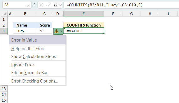
When you encounter an error value in a cell a warning symbol appears, displayed in the image above. Press with mouse on it to see a pop-up menu that lets you get more information about the error.
- The first line describes the error if you press with left mouse button on it.
- The second line opens a pane that explains the error in greater detail.
- The third line takes you to the "Evaluate Formula" tool, a dialog box appears allowing you to examine the formula in greater detail.
- This line lets you ignore the error value meaning the warning icon disappears, however, the error is still in the cell.
- The fifth line lets you edit the formula in the Formula bar.
- The sixth line opens the Excel settings so you can adjust the Error Checking Options.
Here are a few of the most common Excel errors you may encounter.
#NULL error - This error occurs most often if you by mistake use a space character in a formula where it shouldn't be. Excel interprets a space character as an intersection operator. If the ranges don't intersect an #NULL error is returned. The #NULL! error occurs when a formula attempts to calculate the intersection of two ranges that do not actually intersect. This can happen when the wrong range operator is used in the formula, or when the intersection operator (represented by a space character) is used between two ranges that do not overlap. To fix this error double check that the ranges referenced in the formula that use the intersection operator actually have cells in common.
#SPILL error - The #SPILL! error occurs only in version Excel 365 and is caused by a dynamic array being to large, meaning there are cells below and/or to the right that are not empty. This prevents the dynamic array formula expanding into new empty cells.
#DIV/0 error - This error happens if you try to divide a number by 0 (zero) or a value that equates to zero which is not possible mathematically.
#VALUE error - The #VALUE error occurs when a formula has a value that is of the wrong data type. Such as text where a number is expected or when dates are evaluated as text.
#REF error - The #REF error happens when a cell reference is invalid. This can happen if a cell is deleted that is referenced by a formula.
#NAME error - The #NAME error happens if you misspelled a function or a named range.
#NUM error - The #NUM error shows up when you try to use invalid numeric values in formulas, like square root of a negative number.
#N/A error - The #N/A error happens when a value is not available for a formula or found in a given cell range, for example in the VLOOKUP or MATCH functions.
#GETTING_DATA error - The #GETTING_DATA error shows while external sources are loading, this can indicate a delay in fetching the data or that the external source is unavailable right now.
15.2 The formula returns an unexpected value
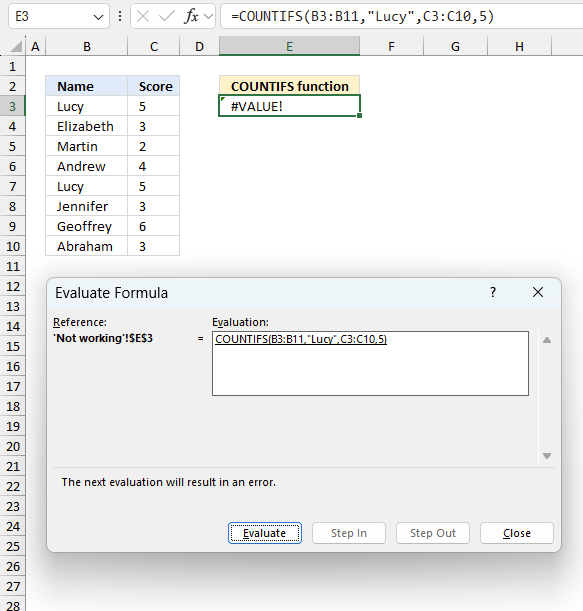
To understand why a formula returns an unexpected value we need to examine the calculations steps in detail. Luckily, Excel has a tool that is really handy in these situations. Here is how to troubleshoot a formula:
- Select the cell containing the formula you want to examine in detail.
- Go to tab “Formulas” on the ribbon.
- Press with left mouse button on "Evaluate Formula" button. A dialog box appears.
The formula appears in a white field inside the dialog box. Underlined expressions are calculations being processed in the next step. The italicized expression is the most recent result. The buttons at the bottom of the dialog box allows you to evaluate the formula in smaller calculations which you control. - Press with left mouse button on the "Evaluate" button located at the bottom of the dialog box to process the underlined expression.
- Repeat pressing the "Evaluate" button until you have seen all calculations step by step. This allows you to examine the formula in greater detail and hopefully find the culprit.
- Press "Close" button to dismiss the dialog box.
There is also another way to debug formulas using the function key F9. F9 is especially useful if you have a feeling that a specific part of the formula is the issue, this makes it faster than the "Evaluate Formula" tool since you don't need to go through all calculations to find the issue..
- Enter Edit mode: Double-press with left mouse button on the cell or press F2 to enter Edit mode for the formula.
- Select part of the formula: Highlight the specific part of the formula you want to evaluate. You can select and evaluate any part of the formula that could work as a standalone formula.
- Press F9: This will calculate and display the result of just that selected portion.
- Evaluate step-by-step: You can select and evaluate different parts of the formula to see intermediate results.
- Check for errors: This allows you to pinpoint which part of a complex formula may be causing an error.
The image above shows cell reference B3:B10 converted to hard-coded value using the F9 key.
Tips!
- View actual values: Selecting a cell reference and pressing F9 will show the actual values in those cells.
- Exit safely: Press Esc to exit Edit mode without changing the formula. Don't press Enter, as that would replace the formula part with the calculated value.
- Full recalculation: Pressing F9 outside of Edit mode will recalculate all formulas in the workbook.
Remember to be careful not to accidentally overwrite parts of your formula when using F9. Always exit with Esc rather than Enter to preserve the original formula. However, if you make a mistake overwriting the formula it is not the end of the world. You can “undo” the action by pressing keyboard shortcut keys CTRL + z or pressing the “Undo” button
15.3 Other errors
Floating-point arithmetic may give inaccurate results in Excel - Article
Floating-point errors are usually very small, often beyond the 15th decimal place, and in most cases don't affect calculations significantly.
'COUNTIFS' function examples
This article explains how to calculate an overlapping time ranges across multiple days. This can be very useful in situations […]
Table of Contents Compare tables: Filter records occurring only in one table Compare two lists and filter unique values where […]
Table of Contents Count cells containing text from list Count entries based on date and time Count cells with text […]
Functions in 'Statistical' category
The COUNTIFS function function is one of 73 functions in the 'Statistical' category.
How to comment
How to add a formula to your comment
<code>Insert your formula here.</code>
Convert less than and larger than signs
Use html character entities instead of less than and larger than signs.
< becomes < and > becomes >
How to add VBA code to your comment
[vb 1="vbnet" language=","]
Put your VBA code here.
[/vb]
How to add a picture to your comment:
Upload picture to postimage.org or imgur
Paste image link to your comment.
Contact Oscar
You can contact me through this contact form