Filter unique distinct records
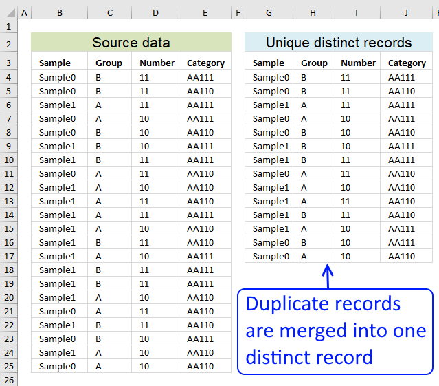
Table of contents
- Filter unique distinct row records
- Filter unique distinct row records but not blanks
- Filter unique distinct row records that does not begin with *string*
- Filter unique distinct row records that begins with *string*
- Filter unique distinct records [Pivot table]
- Filter unique distinct records based on a condition
- Extract unique distinct records based on condition example 2
- Extract unique distinct records from two data sets
Related article:
Extract unique distinct rows sorted from A to Z ignoring blank rows
1. How do I extract unique distinct rows?
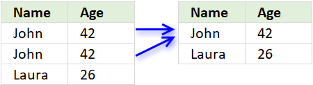
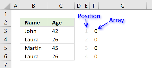
First, let me explain unique distinct records. A record is an entire row in the table, in this example. The picture below displays a small table in columns B and C containing a duplicate record. The table in columns E and F contains unique distinct records only.
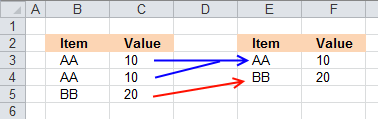
In other words, unique distinct records are all records but duplicate records are removed.
Second, I highly recommend using a pivot table to extract unique distinct records if you are working with a really large data set. A Pivot table is incredibly fast and is also easy to quickly set up and manage.
Third, this post shows you how to construct an array formula that extracts unique distinct records.
Update 10 December 2020, Excel 365 formula:
This is a much smaller regular formula, you can read more about the UNIQUE function here: Extract unique distinct rows
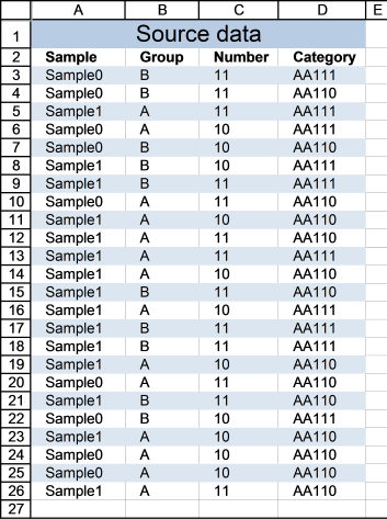
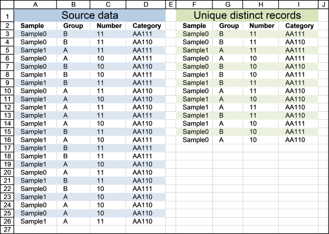
Cell range A3:D26 contains the original list, cell range F3:I16 contains the extracted list. The following formula works for Excel versions prior to Excel 365.
Array formula in cell F3:
How to enter an array formula
- Select cell F3
- Type above formula in cell or formula bar
- Press and hold CTRL + SHIFT simultaneously
- Press Enter once
If you did the steps above correctly, the formula has now a beginning and ending curly bracket, like this {=array_formula}
Don't enter these characters yourself, they appear automatically if you did this right.
How to copy formula
Copy cell F3 and paste it to cells to the right, as far as needed. Then copy cells and paste them down, as far as needed.
Explaining array formula in cell F3
You can easily follow along while I go through this array formula, go to tab "Formulas" on the ribbon. Select cell F3 then press with left mouse button on "Evaluate Formula" button. Press with left mouse button on "Evaluate" button to move to next step.
Step 1 - Identify rows with unique records
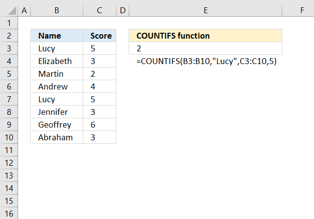
The COUNTIFS function counts the number of cells specified by a given set of conditions or criteria
COUNTIFS($F$2:$F2, $A$3:$A$26, $G$2:$G2, $B$3:$B$26, $H$2:$H2, $C$3:$C$26, $I$2:$I2, $D$3:$D$26)
becomes
COUNTIFS($A$28:$A28, {"Sample0"; "Sample0"; "Sample1"; "Sample0"; "Sample0"; "Sample1"; "Sample1"; "Sample0"; "Sample1"; "Sample1"; "Sample1"; "Sample1"; "Sample1"; "Sample1"; "Sample1"; "Sample1"; "Sample1"; "Sample0"; "Sample1"; "Sample0"; "Sample1"; "Sample0"; "Sample0"; "Sample1"}, $B$28:$B28, {"B";"B";"A";"A";"B";"B"; "B";"A";"A";"A";"A";"A";"B";"A";"B"; "B";"A";"A";"B";"B";"A";"A";"A";"A"}, $C$28:$C28, {11; 11; 11; 10; 10; 10; 11; 11; 10; 11; 11; 10; 11; 10; 11; 11; 10; 11; 11; 10; 10; 10; 10; 11}, $D$28:$D28, {"AA111"; "AA110"; "AA111"; "AA111"; "AA110"; "AA111"; "AA111"; "AA110"; "AA110"; "AA110"; "AA111"; "AA110"; "AA110"; "AA111"; "AA111"; "AA111"; "AA110"; "AA110"; "AA110"; "AA111"; "AA110"; "AA110"; "AA110"; "AA110"})
becomes
COUNTIFS("Sample", {"Sample0"; "Sample0"; "Sample1"; "Sample0"; "Sample0"; "Sample1"; "Sample1"; "Sample0"; "Sample1"; "Sample1"; "Sample1"; "Sample1"; "Sample1"; "Sample1"; "Sample1"; "Sample1"; "Sample1"; "Sample0"; "Sample1"; "Sample0"; "Sample1"; "Sample0"; "Sample0"; "Sample1"}, "Group", {"B";"B";"A";"A";"B";"B"; "B";"A";"A";"A";"A";"A";"B";"A";"B"; "B";"A";"A";"B";"B";"A";"A";"A";"A"}, "Number", {11; 11; 11; 10; 10; 10; 11; 11; 10; 11; 11; 10; 11; 10; 11; 11; 10; 11; 11; 10; 10; 10; 10; 11}, "Category", {"AA111"; "AA110"; "AA111"; "AA111"; "AA110"; "AA111"; "AA111"; "AA110"; "AA110"; "AA110"; "AA111"; "AA110"; "AA110"; "AA111"; "AA111"; "AA111"; "AA110"; "AA110"; "AA110"; "AA111"; "AA110"; "AA110"; "AA110"; "AA110"})
and returns
{0; 0; 0; 0; 0; 0; 0; 0; 0; 0; 0; 0; 0; 0; 0; 0; 0; 0; 0; 0; 0; 0; 0; 0}
Step 2 - Find relative position of a unique record
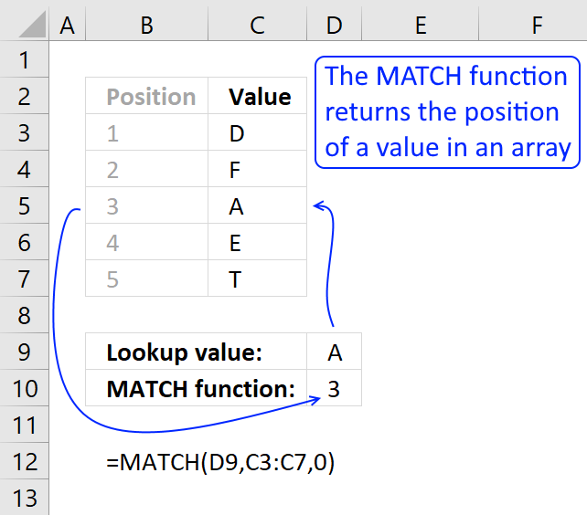
The MATCH function returns the relative position of an item in an array that matches a specified value
MATCH(0, COUNTIFS($F$2:$F2, $A$3:$A$26, $G$2:$G2, $B$3:$B$26, $H$2:$H2, $C$3:$C$26, $I$2:$I2, $D$3:$D$26), 0)
becomes
MATCH(0, {0; 0; 0; 0; 0; 0; 0; 0; 0; 0; 0; 0; 0; 0; 0; 0; 0; 0; 0; 0; 0; 0; 0; 0}, 0)
and returns 1.
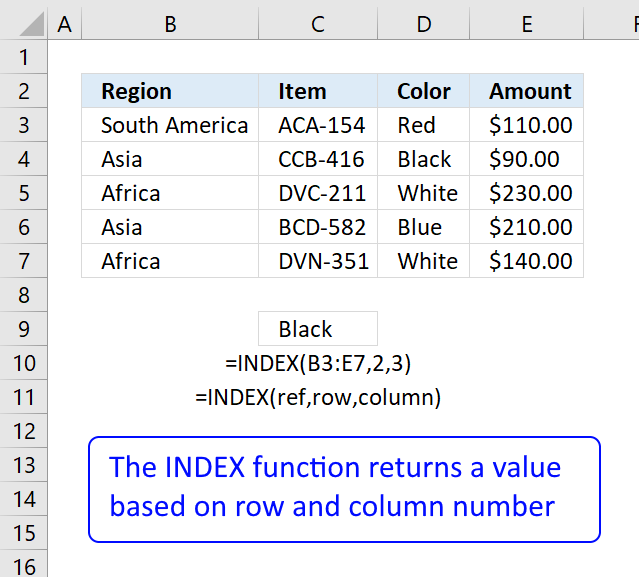
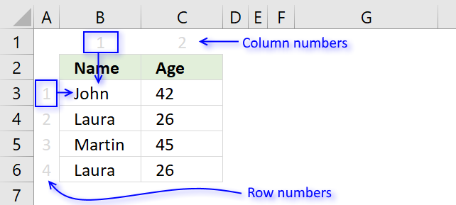
Step 3 - Return a value of the cell at the intersection of a particular row and column
The INDEX function returns a value or reference of the cell at the intersection of a particular row and column, in a given range
INDEX($A$3:$D$26, MATCH(0, COUNTIFS($F$2:$F2, $A$3:$A$26, $G$2:$G2, $B$3:$B$26, $H$2:$H2, $C$3:$C$26, $I$2:$I2, $D$3:$D$26), 0), COLUMN(A1))
becomes
INDEX($A$3:$D$26, 1, COLUMN(A1))
becomes
INDEX($A$3:$D$26, 1, 1)
becomes
INDEX({"Sample0", "B", 11, "AA111"; "Sample0", "B", 11, "AA110"; "Sample1", "A", 11, "AA111"; "Sample0", "A", 10, "AA111"; "Sample0", "B", 10, "AA110"; "Sample1", "B", 10, "AA111"; "Sample1", "B", 11, "AA111"; "Sample0", "A", 11, "AA110"; "Sample1", "A", 10, "AA110"; "Sample1", "A", 11, "AA110"; "Sample1", "A", 11, "AA111"; "Sample1", "A", 10, "AA110"; "Sample1", "B", 11, "AA110"; "Sample1", "A", 10, "AA111"; "Sample1", "B", 11, "AA111"; "Sample1", "B", 11, "AA111"; "Sample1", "A", 10, "AA110"; "Sample0", "A", 11, "AA110"; "Sample1", "B", 11, "AA110"; "Sample0", "B", 10, "AA111"; "Sample1", "A", 10, "AA110"; "Sample0", "A", 10, "AA110"; "Sample0", "A", 10, "AA110"; "Sample1", "A", 11, "AA110"}, 1, 1)
and returns "Sample0" in cell F3.
Related articles
Recommended articles

First, let me explain the difference between unique values and unique distinct values, it is important you know the difference […]
2. Filter unique distinct row records but not blanks
The image below shows you a data table in column A:D. Unfortunately, it has some blank rows, however, the formula below takes handles this issue.
![]()
Update 11 December 2020, Excel 365 formula in cell F3:
This is a much smaller formula also entered as a regular formula, you can read more about the UNIQUE function here: Extract unique distinct rows ignoring blank rows
The following array formula in cell F3 works with previous Excel versions:
3. Extract unique distinct rows that don't begin with a given string
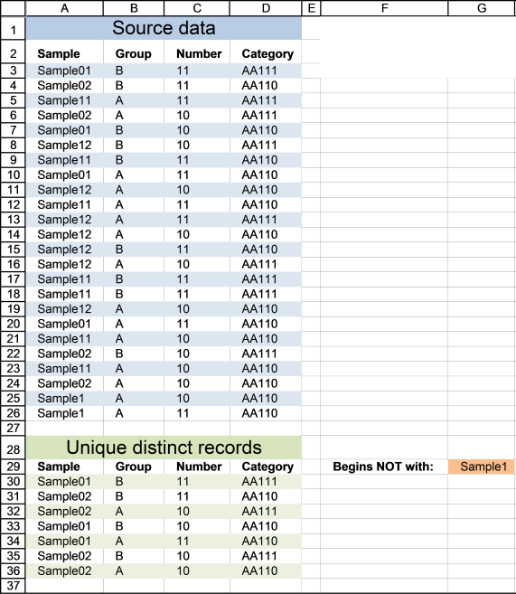
This example lets you specify a string and a record is shown in cell range A30:D36 if it does NOT match the beginning characters in column A and it is NOT a DUPLICATE record.
Update 11 December 2020, Excel 365 formula in cell A30:
The formula below is for previous Excel versions.
Array formula in cell A30:
4. Extract unique distinct rows that begin with *string*
If you are looking for records that begin with *string*, see this formula. Note that the formula looks for values in col A that begins with a specific text string.
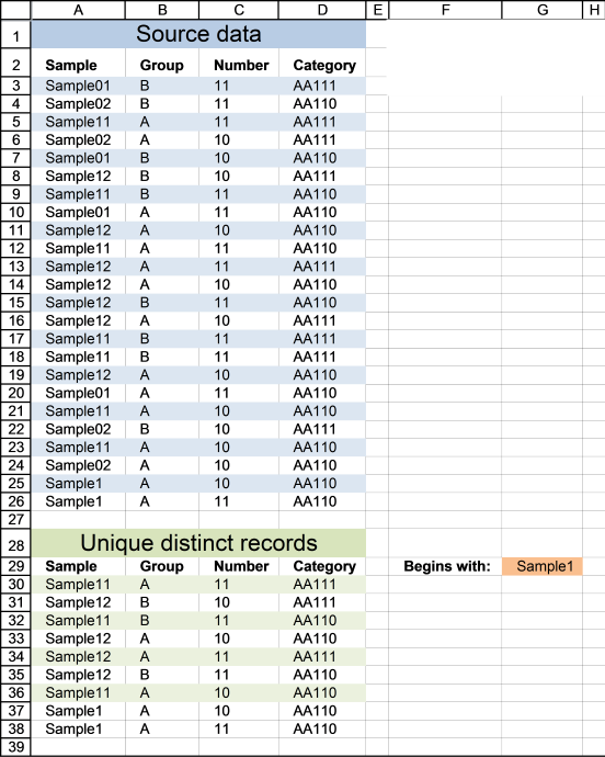
Update 11 December 2020, Excel 365 formula in cell A30:
The formula below is for previous Excel versions.
Array formula in cell A30:
6. Filter unique distinct records with a condition

If Tea and Coffee has Americano,it will only return Americano once and not twice. I am looking for a unique distinct list based on each condition.
I remember reading that Excel has difficulty with these type of or conditions in arrays.
Answer:
Array formula in cell C19:
To enter an array formula, type the formula in a cell then press and hold CTRL + SHIFT simultaneously, now press Enter once. Release all keys.
The formula bar now shows the formula with a beginning and ending curly bracket telling you that you entered the formula successfully. Don't enter the curly brackets yourself.
Excel 365 dynamic array formula in cell C19:
=UNIQUE(FILTER(C5:D11,COUNTIF(C13:C14,C5:C11)))
Copy array formula
- Select cell C19
- Copy cell (Ctrl + c)
- Select cell range C19:D22
- Paste (Ctrl + v)
How the array formula in cell C19 works
Step 1 - Identify unique distinct records
COUNTIFS($C$18:C18, $C$5:$C$11, $D$18:D18, $D$5:$D$11)
becomes
COUNTIFS("Category", {"Coffee";"Coffee";"Coffee";"Coffee";"tea";"juice";"tea"}, "Item", {"Espresso";"Espresso";"Americano";"Americano";"Americano";"Florida";"English"},)
and returns {0;0;0;0;0;0;0}
Recommended articles
Checks multiple conditions against the same number of cell ranges and counts how many times all criteria are met.
Step 2 - Filter records with condition
COUNTIF($C$13:$C$14, $C$5:$C$11)=0
becomes
COUNTIF({"Coffee"; "tea"}, {"Coffee"; "Coffee"; "Coffee"; "Coffee"; "tea"; "juice"; "tea"})=0
and returns {FALSE; FALSE; FALSE; FALSE; FALSE; TRUE; FALSE}
Recommended articles

Counts the number of cells that meet a specific condition.
Step 3 - Match filtered records
MATCH(0, COUNTIFS($C$18:C18, $C$5:$C$11, $D$18:D18, $D$5:$D$11)+(COUNTIF($C$13:$C$14, $C$5:$C$11)=0), 0)
becomes
MATCH(0, {0;0;0;0;0;0;0}+{FALSE; FALSE; FALSE; FALSE; FALSE; TRUE; FALSE}, 0)
becomes
MATCH(0, {0;0;0;0;0;1;0},0)
and returns 1.
Recommended articles
Identify the position of a value in an array.
Step 4 - Return a value or reference of the cell at the intersection of a particular row and column
INDEX($C$5:$D$11, MATCH(0, COUNTIFS($C$18:C18, $C$5:$C$11, $D$18:D18, $D$5:$D$11)+(COUNTIF($C$13:$C$14, $C$5:$C$11)=0), 0), COLUMN(A1))
becomes
INDEX({"Coffee", "Espresso";"Coffee", "Espresso";"Coffee", "Americano";"Coffee", "Americano";"tea", "Americano";"juice", "Florida";"tea", "English"}, 1, 1)
and returns "Coffee" in cell C19.
Recommended articles
Gets a value in a specific cell range based on a row and column number.
Tip! Did you know that a pivot table can easily extract unique distinct records too?
Recommended articles
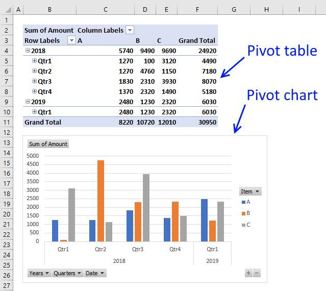
A pivot table allows you to examine data more efficiently, it can summarize large amounts of data very quickly and is very easy to use.
How to remove errors
IFERROR(value, value_if_error) returns value_if_error if expression is an error and the value of the expression itself otherwise
The array formula becomes:
7. Extract unique distinct records based on condition, example 2
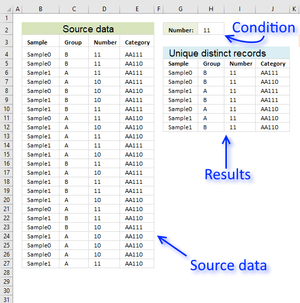
In this section, I want to show you how to narrow that search down a bit further. This time I want to search for unique distinct records based on a condition that must match. I want to extract for unique distinct records with column C containing value 11.
Array formula in G6:
To enter an array formula, type the formula in cell G6 then press and hold CTRL + SHIFT simultaneously, now press Enter once. Release all keys.
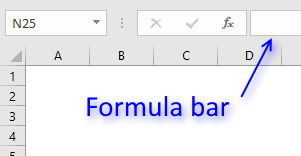 The formula bar now shows the formula with a beginning and ending curly bracket telling you that you entered the formula successfully.
Don't enter the curly brackets yourself, they appear automatically.
Excel 365 dynamic array formula in cell G6:
Explaining formula in cell G6
First, let me explain what a unique distinct record is. A record is an entire row in the table, in this example. The picture below displays a small table in column B and C containing a duplicate record. The table in column E and F contains only unique distinct records.
In other words, unique distinct records are all records but duplicate records are removed. The record in cell range B4:C4 is removed.
Step 1 - Check if records have been displayed
The COUNTIFS function lets you count values combined which is perfect when it comes to counting data records. The following part of the formula checks if previous records in the list has been displayed, if a record has been shown the corresponding value in the array returns 1 and if not 0 (zero).
COUNTIFS($G$5:$G5, $B$4:$B$27, $H$5:$H5, $C$4:$C$27, $I$5:$I5, $D$4:$D$27, $J$5:$J5, $E$4:$E$27)
returns {0; 0; 0; 0; 0; 0; 0; 0; 0; 0; 0; 0; 0; 0; 0; 0; 0; 0; 0; 0; 0; 0; 0; 0}.
This means that no record has been displayed yet in the list, remember that we are checking the formula in cell G6.
Step 2 - Make sure that only records with the condition met are filtered
The COUNTIF function lets you build an array that indicates which records meet the condition.
COUNTIF($H$2,$D$4:$D$27)=0
becomes
{1;1;1;0;0;0;1;1;0;1;1;0;1;0;1;1;0;1;1;0;0;0;0;1}=0
and returns {FALSE; FALSE; FALSE; TRUE; TRUE; TRUE; FALSE; FALSE; TRUE; FALSE; FALSE; TRUE; FALSE; TRUE; FALSE; FALSE; TRUE; FALSE; FALSE; TRUE; TRUE; TRUE; TRUE; FALSE}.
Step 3 - Add arrays
COUNTIFS($G$5:$G5, $B$4:$B$27, $H$5:$H5, $C$4:$C$27, $I$5:$I5, $D$4:$D$27, $J$5:$J5, $E$4:$E$27)+(COUNTIF($H$2,$D$4:$D$27)=0)
becomes
{0; 0; 0; 0; 0; 0; 0; 0; 0; 0; 0; 0; 0; 0; 0; 0; 0; 0; 0; 0; 0; 0; 0; 0} + {FALSE; FALSE; FALSE; TRUE; TRUE; TRUE; FALSE; FALSE; TRUE; FALSE; FALSE; TRUE; FALSE; TRUE; FALSE; FALSE; TRUE; FALSE; FALSE; TRUE; TRUE; TRUE; TRUE; FALSE}
and returns {0;0;0;1;1;1;0;0;1;0;0;1;0;1;0;0;1;0;0;1;1;1;1;0}.
Step 4 - Find the position of the first 0 (zero) in the array
To be able to get the record we need the formula needs to know where the first record is that not yet has been shown. The MATCH function lets you find the position of the first 0 (zero) in the array.
MATCH(0, COUNTIFS($G$5:$G5, $B$4:$B$27, $H$5:$H5, $C$4:$C$27, $I$5:$I5, $D$4:$D$27, $J$5:$J5, $E$4:$E$27)+(COUNTIF($H$2,$D$4:$D$27)=0), 0)
becomes
MATCH(0, {0;0;0;1;1;1;0;0;1;0;0;1;0;1;0;0;1;0;0;1;1;1;1;0}, 0)
and returns 1.
Step 5 - Return the first value from the first record
The INDEX function lets you get a value from the worksheet based on a row number and column number.
INDEX($B$4:$E$27, MATCH(0, COUNTIFS($G$5:$G5, $B$4:$B$27, $H$5:$H5, $C$4:$C$27, $I$5:$I5, $D$4:$D$27, $J$5:$J5, $E$4:$E$27)+(COUNTIF($H$2,$D$4:$D$27)=0), 0), COLUMN(A1))
becomes
INDEX($B$4:$E$27, 1, COLUMN(A1))
becomes
INDEX($B$4:$E$27, 1, 1)
and returns "Sample0" in cell G6.
Get Excel *.xlsx file
Extract unique distinct records based on a condition.xlsx
8. Extract unique distinct records from two data sets
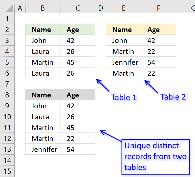
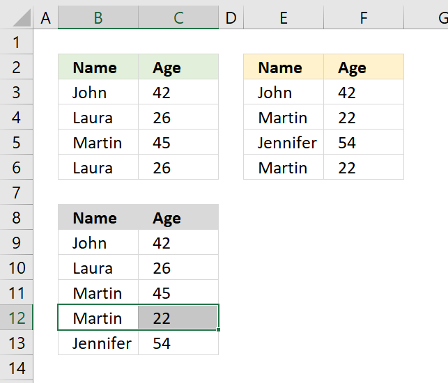
The picture above shows an array formula in cell B9:C13 that extracts unique distinct records from two tables in cell range B3:C6 and E3:F6.
If a record exists in both tables only one record is returned by the formula. If a record exists multiple times in one table only one record is returned by the formula.
Example, John 42 exists in both tables, however, the formula returns only one instance of John 42.
Laura 26 exists multiple times but only in the first table, the formula returns only one record of Laura 26.
Excel 365 dynamic array formula in cell B9:
Array formula in cell B9 for older Excel versions:
To enter an array formula, type the formula in cell B9 then press and hold CTRL + SHIFT simultaneously, now press Enter once. Release all keys.
The formula bar now shows the formula with a beginning and ending curly bracket telling you that you entered the formula successfully.
Don't enter the curly brackets yourself, they appear automatically.
What is a unique distinct record?
Unique distinct records are all records except duplicates merged into one distinct value.
In other words, duplicate records are removed.
Explaining the formula in cell B9
Use the "Evaluate Formula" tool to examine the calculation steps in greater detail.
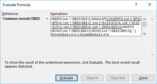 Go to tab "Formula" on the ribbon, press with left mouse button on "Evaluate Formula" button to start the tool.
Then press with left mouse button on the "Evaluate" button to see the next step in the calculation, this will make it easier to understand how the formula works.
Step 1 - Count previous records against table 1
The COUNTIFS function allows you to count how many times a record exists in a table.
The previous values in cell B9 are the values in B8 and C8.
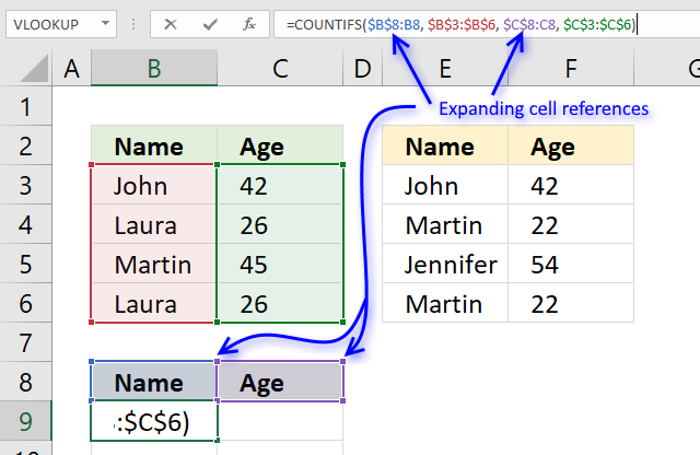
The first argument $B$8:B8 in the COUNTIFS function has both absolute and relative cell references, this allows the formula to automatically expand when you copy it and paste to cells below.
"Name" and "Age" is not found in cell range B3:C6 so the COUNTIFS function returns 0 (zero) for each record.
COUNTIFS($B$8:B8, $B$3:$B$6, $C$8:C8, $C$3:$C$6)
becomes
=COUNTIFS("Name", {"John";"Laura";"Martin";"Laura"}, "Age", {42;26;45;26})
and returns {0;0;0;0}. There are four records and the function returns an array containing 4 values (zeros).
Step 2 - Find the first instance of 0 (zero) in the array
The MATCH function allows you to identify which record to return next.
MATCH(0, COUNTIFS($B$8:B8, $B$3:$B$6, $C$8:C8, $C$3:$C$6), 0)
becomes
MATCH(0, {0;0;0;0}, 0)
and returns 1. The first instance of 0 (zero) is found in position 1 in the array.
Step 3 - Return value from a record
The INDEX function lets get a specific value using a row and column number.
The MATCH function calculates the row number we need to get the correct value, however, the COLUMNS function keeps track of which value in the record to get.
The COLUMNS function calculates the number of columns in a cell reference, the cell reference used here $A$1:A1 is also expanding when the formula is copied to other cells.
COLUMNS($A$1:A1) returns 1.
INDEX($B$3:$C$6, MATCH(0, COUNTIFS($B$8:B8, $B$3:$B$6, $C$8:C8, $C$3:$C$6), 0),COLUMNS($A$1:A1))
becomes
INDEX($B$3:$C$6, 1, COLUMNS($A$1:A1))
becomes
INDEX($B$3:$C$6, 1, 1) and returns John in cell B9.
Step 4 - IFNA function points the calculation in a new direction
Step 1 to 3 explains how the formula extracts unique distinct records from the first table.
The first part of the formula returns a #N/A error when there are no records left in table 1 to extract.
The IFNA function points the calculation to part2 when the error occurs.
The second part of the formula does the exact same thing as the first part except that the cell references this time points to the second table.
The picture above shows that the two last records are extracted from the second table.
Get Excel *.xlsx file
Extract unique distinct records from two data sets.xlsx
Unique distinct records category
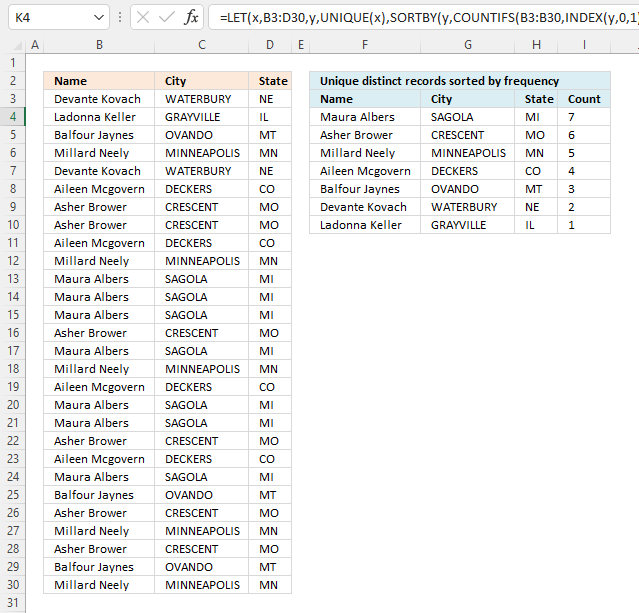
This article demonstrates how to sort records in a data set based on their count meaning the formula counts each […]
This article demonstrates two ways to extract unique and unique distinct rows from a given cell range. The first one […]
Excel categories
5 Responses to “Filter unique distinct records”
How to comment
How to add a formula to your comment
<code>Insert your formula here.</code>
Convert less than and larger than signs
Use html character entities instead of less than and larger than signs.
< becomes < and > becomes >
How to add VBA code to your comment
[vb 1="vbnet" language=","]
Put your VBA code here.
[/vb]
How to add a picture to your comment:
Upload picture to postimage.org or imgur
Paste image link to your comment.
[...] Filed in Excel on Feb.02, 2009. Email This article to a Friend In a previous article “Automatically filter unique row records from multiple columns“, i presented a solution to filter out unique values from several columns. In this article i [...]
[...] We can verify the calculation by extracting all unqiue distinct records from the above table. I am using a formula from this blog article: Filter unique distinct row records in excel 2007 [...]
Oscar, this works great. Keep up the great work.
When I tried the workbook that was uploaded to this post-reply and pressed with left mouse button on the formula bar for cell C19 and hit 'ENTER' (without actually changing anything) and I get an #N/A record.
I'm running excel 2010, so I can only assume that the code in cell C19 'may' not work in 2010? Could this be possible? If so, can you help me with code that would work in Excel 2010??
Carlos,
When I tried the workbook that was uploaded to this post-reply and pressed with left mouse button on the formula bar for cell C19 and hit 'ENTER' (without actually changing anything) and I get an #N/A record.
That is one of the disadvantages with array formulas. If you edit an array formula (even though you don´t do any changes) you must enter it as an array formula. See: How to create an array formula, above.
I'm running excel 2010, so I can only assume that the code in cell C19 'may' not work in 2010? Could this be possible? If so, can you help me with code that would work in Excel 2010??
It works in excel 2010.