Unique distinct records sorted based on count or frequency

This article demonstrates how to sort records in a data set based on their count meaning the formula counts each record and returns a unique distinct list sorted based on a count from large to small.
For example, the first record is shown in cell range F4:H4. The count is in cell I4, it corresponds to the number of times the record is repeated in cell range B3:D30.
This tells us that the record is displayed seven times and is the most repeated record, it is at the very top of the list.
I will also show a much smaller formula that works only in Excel 365, that formula is entered as a regular formula despite the fact that it returns an array of values.
Lastly, a solution for a Pivot Table is also demonstrated.
Table of Contents
1. Unique distinct records sorted based on count or frequency - Excel 365
This formula extracts unique distinct rows in cell range B3:D30 and returns a sorted list based on how many times each row is repeated in B3:D30 from large to small.
Excel 365 formula in cell F4:
You need to change the formula if the data source has more or fewer columns than this example. A data source containing two columns B3:C30 shrinks the formula to this:
2.1 Explaining the formula in cell F4
Step 1 - Extract unique distinct records
The UNIQUE function extracts unique distinct values or records.
UNIQUE(array,[by_col],[exactly_once])
UNIQUE(B3:D30)
returns the following data set, see image below.

Step 2 - Extract column from unique distinct records
The INDEX function lets you extract an entire column from an array. This is possible if you use 0 (zero) in the row argument meaning all rows will be extracted. The third argument will lets you choose which column to extract.
Number 1 extracts the first column in the array.
INDEX(array, [row_num], [column_num], [area_num])
INDEX(UNIQUE(B3:D30),0,1)
returns
{"Devante Kovach"; "Ladonna Keller"; "Balfour Jaynes"; "Millard Neely"; "Aileen Mcgovern"; "Asher Brower"; "Maura Albers"}.
Step 3 - Count records
The COUNTIFS function calculates the number of cells across multiple ranges that equals all given conditions.
COUNTIFS(criteria_range1, criteria1, [criteria_range2, criteria2]…)
COUNTIFS(B3:B30, INDEX(UNIQUE(B3:D30), 0, 1), C3:C30, INDEX(UNIQUE(B3:D30), 0, 2), D3:D30, INDEX(UNIQUE(B3:D30), 0, 3))
returns {2; 1; 3; 5; 4; 6; 7}.

The array of numbers is displayed in the image above, each number corresponds to the record on the same row. We can use this relationship to sort the records based on the count.
Step 4 - Sort by count
The SORTBY function lets you sort values from a cell range or array based on a corresponding cell range or array. It sorts values by column but keeps rows.
SORTBY(array, by_array1, [sort_order1], [by_array2, sort_order2],…)
SORTBY(UNIQUE(B3:D30), COUNTIFS(B3:B30, INDEX(UNIQUE(B3:D30), 0, 1), C3:C30, INDEX(UNIQUE(B3:D30), 0, 2), D3:D30, INDEX(UNIQUE(B3:D30), 0, 3)), -1)
becomes
SORTBY(UNIQUE(B3:D30), {2; 1; 3; 5; 4; 6; 7}, -1)
and returns the following array:

The records are now sorted based on the count from large to small.
Step 5 - Shorten formula
The formula can be shortened using the LET function. The LET function lets you name intermediate calculation results which can shorten formulas considerably and improve performance.
LET(name1, name_value1, calculation_or_name2, [name_value2, calculation_or_name3...])
SORTBY(UNIQUE(B3:D30), COUNTIFS(B3:B30, INDEX(UNIQUE(B3:D30), 0, 1), C3:C30, INDEX(UNIQUE(B3:D30), 0, 2), D3:D30, INDEX(UNIQUE(B3:D30), 0, 3)), -1)
UNIQUE(B3:D30) is used a lot in the formula.
y - UNIQUE(B3:D30)
LET(y, UNIQUE(B3:D30), SORTBY(y, COUNTIFS(B3:B30, INDEX(y, 0, 1), C3:C30, INDEX(y, 0, 2), D3:D30, INDEX(y, 0, 3)), -1))
Get Excel *.xlsx file
2. Unique distinct records sorted based on count - Pivot Table

This example demonstrates how to count unique distinct records in a Pivot Table. The image above shows a Pivot Table containing nine different records sorted based on the count, here is how I created this Pivot Table calculation.
2.1 Add a helper column

The image above shows the source data I am using in this example. The Pivot Table can calculate the count of unique distinct values but not unique distinct records as far as I know.
We need a helper column that merges all values row by row.
Formula in cell E3:
Copy cell E3 and paste to cells below as far as needed.
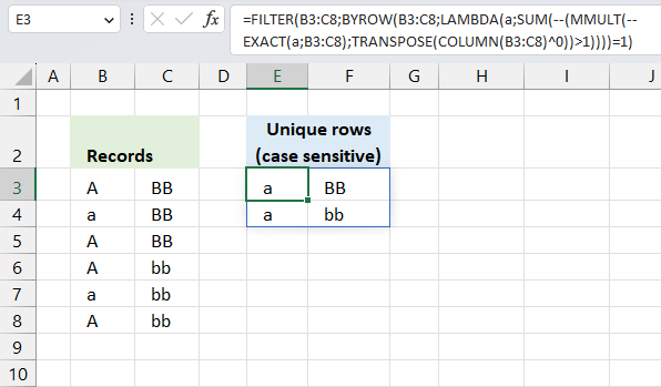
This formula uses a delimiting character that is not used in the original data source. It is important that you choose a "unique" delimiting character not used in the original data source in order to be able to count unique distinct records.
Here is an example that shows what might happen if we don't choose a "unique" delimiting character. For example, Value "A" and "BB" returns "ABB" if we join the values without a delimiting character.
Value "AB" and "B" also return "ABB", however, the record is different. Let's try this example with a delimiting character "|". "A" and "BB" returns "A|BB" and "AB" and "B" returns ""AB|B".

2.2 Insert a Pivot Table

- Select any cell in the data. I chose cell E3, see the image above.
- Go to tab "Insert" on the ribbon.
- Press with left mouse button on the "Pivot Table" button.
- A dialog box appears, select "Existing Worksheet".
- Select a destination cell by press with left mouse button oning the arrow button. I chose cell G2, see the image above.
- Press with left mouse button on the check box "Add this data to the Data Model".
- Press with left mouse button on "OK" button to apply changes.

An empty pivot table appears in cell G2, see the image above.
2.4 Configure Pivot Table

- Select any cell in the empty Pivot Table.
- A settings pane appears to the right, see the image above.
- Press and hold with left mouse button on "Join" located in the PivotTable Fields.
- Drag with mouse to "Rows" field.
- Repeat step 3 and then drag to the "Values" field, see the image above.
2.5 Sort Pivot Table based on the count

- Press with right mouse button on on any cell in the column "Count of Join".
- A popup menu appears, press with left mouse button on "Sort".
- Another popup menu appears, press with left mouse button on "Sort Largest to Smallest".
The pivot table now shows unique distinct records sorted by count.
Get Excel file
Unique distinct records sorted by frequencyv3
3. Unique distinct records sorted based on count or frequency

How can you use large with multiple criteria?? Example looking for top 5 of a list based on name, state and city..
The formula entered in cell E3 extracts unique distinct records sorted based on frequency or count.
Array formula in cell E3:
1.1 How to enter an array formula
- Copy above array formula.
- Select cell E3
- Paste array formula to cell E3
- Press and hold CTRL + SHIFT simultaneously.
- Press Enter once.
- Release all keys.
If you did it right the formula is now enclosed with curly brackets, don't enter these characters yourself. They appear automatically if you followed the above steps.
1.2 How to copy array formula and paste to remaining cells
- Select cell E3
- Copy cell (not formula). (CTRL + c)
- Select cell range F3:G3
- Paste to cell range F3:G3. (CTRL + v)
- Select cell range E3:G3.
- Copy cells (not formulas). (CTRL + c)
- Select cell range E4:G9.
- Paste to cell range E4:G9. (CTRL + v)
Regular formula in cell H3:
1.3 Explaining array formula in cell E3
Step 1 - Identify records not displayed yet
The COUNTIFS function allows you to count cells based on multiple conditions, this makes it ideal for identifying unique distinct records, one condition corresponds to one value in the record.
If you have three values in one record then the COUNTIFS function contains three conditions or six arguments. Each condition has two arguments, the first argument in each pair is a growing cell reference meaning it expands when you copy the cell and paste to cells below.
COUNTIFS($E$2:E2,$A$2:$A$29,$F$2:F2,$B$2:$B$29,$G$2:G2,$C$2:$C$29)=0
becomes
{0; 0; 0; 0; 0; 0; 0; 0; 0; 0; 0; 0; 0; 0; 0; 0; 0; 0; 0; 0; 0; 0; 0; 0; 0; 0; 0; 0}=0
and returns
{TRUE; TRUE; TRUE; TRUE; TRUE; TRUE; TRUE; TRUE; TRUE; TRUE; TRUE; TRUE; TRUE; TRUE; TRUE; TRUE; TRUE; TRUE; TRUE; TRUE; TRUE; TRUE; TRUE; TRUE; TRUE; TRUE; TRUE; TRUE}.
This makes sense since no values have been displayed yet by the formula in cells above cell E3.
Step 2 - Calculate record frequency
The COUNTIFS function also lets you count identical records, by using the IF function we can convert the boolean values to the corresponding count if TRUE and blank "" if FALSE.
IF(COUNTIFS($E$2:E2, $A$2:$A$29, $F$2:F2, $B$2:$B$29, $G$2:G2, $C$2:$C$29)=0, COUNTIFS($A$2:$A$29, $A$2:$A$29, $B$2:$B$29, $B$2:$B$29, $C$2:$C$29, $C$2:$C$29), "")
becomes
IF({TRUE; TRUE; TRUE; TRUE; TRUE; TRUE; TRUE; TRUE; TRUE; TRUE; TRUE; TRUE; TRUE; TRUE; TRUE; TRUE; TRUE; TRUE; TRUE; TRUE; TRUE; TRUE; TRUE; TRUE; TRUE; TRUE; TRUE; TRUE}, COUNTIFS($A$2:$A$29, $A$2:$A$29, $B$2:$B$29, $B$2:$B$29, $C$2:$C$29, $C$2:$C$29), "")
becomes
IF({TRUE; TRUE; TRUE; TRUE; TRUE; TRUE; TRUE; TRUE; TRUE; TRUE; TRUE; TRUE; TRUE; TRUE; TRUE; TRUE; TRUE; TRUE; TRUE; TRUE; TRUE; TRUE; TRUE; TRUE; TRUE; TRUE; TRUE; TRUE}, {2; 1; 3; 5; 2; 4; 6; 6; 4; 5; 7; 7; 7; 6; 7; 5; 4; 7; 7; 6; 4; 7; 3; 6; 5; 6; 3; 5}, "")
and returns
{2; 1; 3; 5; 2; 4; 6; 6; 4; 5; 7; 7; 7; 6; 7; 5; 4; 7; 7; 6; 4; 7; 3; 6; 5; 6; 3; 5}.
The first value in the array above corresponds to the first record (row) in cell range $A$2:$C$29, thus 2 tells us that there is an identical record somewhere in cell range $A$2:$C$29. If we examine the list above you can see that the first record (row 2) is identical to the record in row 6.
Row 6 is the fifth value in the array above, that value must also be 2 if the formula works as intended. Yes, the fifth value is also 2.
Step 3 - Extract largest number from array
The LARGE function lets you extract the k-th largest value in a cell range or array, in this case, we are looking for the largest value and k is therefore 1.
LARGE(IF(COUNTIFS($E$2:E2, $A$2:$A$29, $F$2:F2, $B$2:$B$29, $G$2:G2, $C$2:$C$29)=0, COUNTIFS($A$2:$A$29, $A$2:$A$29, $B$2:$B$29, $B$2:$B$29, $C$2:$C$29, $C$2:$C$29), ""), 1)
becomes
LARGE({2; 1; 3; 5; 2; 4; 6; 6; 4; 5; 7; 7; 7; 6; 7; 5; 4; 7; 7; 6; 4; 7; 3; 6; 5; 6; 3; 5},1)
and returns 7.
Step 4 - Find position of largest value
The MATCH function returns the relative position of a value in an array or cell range. The array we match against is the frequency numbers multiplied with an array with boolean values that indicates if a record has already been shown in cells above the current cell.
MATCH(LARGE(IF(COUNTIFS($E$2:E2,$A$2:$A$29,$F$2:F2,$B$2:$B$29,$G$2:G2,$C$2:$C$29)=0,COUNTIFS($A$2:$A$29,$A$2:$A$29,$B$2:$B$29,$B$2:$B$29,$C$2:$C$29,$C$2:$C$29),""),1),COUNTIFS($A$2:$A$29,$A$2:$A$29,$B$2:$B$29,$B$2:$B$29,$C$2:$C$29,$C$2:$C$29)*(COUNTIFS($E$2:E2,$A$2:$A$29,$F$2:F2,$B$2:$B$29,$G$2:G2,$C$2:$C$29)=0),0)
becomes
MATCH(7,COUNTIFS($A$2:$A$29,$A$2:$A$29,$B$2:$B$29,$B$2:$B$29,$C$2:$C$29,$C$2:$C$29)*(COUNTIFS($E$2:E2,$A$2:$A$29,$F$2:F2,$B$2:$B$29,$G$2:G2,$C$2:$C$29)=0),0)
becomes
MATCH(7,{2; 1; 3; 5; 2; 4; 6; 6; 4; 5; 7; 7; 7; 6; 7; 5; 4; 7; 7; 6; 4; 7; 3; 6; 5; 6; 3; 5}*(COUNTIFS($E$2:E2,$A$2:$A$29,$F$2:F2,$B$2:$B$29,$G$2:G2,$C$2:$C$29)=0),0)
becomes
MATCH(7,{2; 1; 3; 5; 2; 4; 6; 6; 4; 5; 7; 7; 7; 6; 7; 5; 4; 7; 7; 6; 4; 7; 3; 6; 5; 6; 3; 5}*{TRUE; TRUE; TRUE; TRUE; TRUE; TRUE; TRUE; TRUE; TRUE; TRUE; TRUE; TRUE; TRUE; TRUE; TRUE; TRUE; TRUE; TRUE; TRUE; TRUE; TRUE; TRUE; TRUE; TRUE; TRUE; TRUE; TRUE; TRUE},0)
becomes
MATCH(7,{2; 1; 3; 5; 2; 4; 6; 6; 4; 5; 7; 7; 7; 6; 7; 5; 4; 7; 7; 6; 4; 7; 3; 6; 5; 6; 3; 5},0)
and returns 11. Number 7 is found int the 11-th position in the array.
Step 5 - Return value based on position
INDEX($A$2:$C$29,MATCH(LARGE(IF(COUNTIFS($E$2:E2,$A$2:$A$29,$F$2:F2,$B$2:$B$29,$G$2:G2,$C$2:$C$29)=0,COUNTIFS($A$2:$A$29,$A$2:$A$29,$B$2:$B$29,$B$2:$B$29,$C$2:$C$29,$C$2:$C$29),""),1),COUNTIFS($A$2:$A$29,$A$2:$A$29,$B$2:$B$29,$B$2:$B$29,$C$2:$C$29,$C$2:$C$29)*(COUNTIFS($E$2:E2,$A$2:$A$29,$F$2:F2,$B$2:$B$29,$G$2:G2,$C$2:$C$29)=0),0),COLUMN(A1))
becomes
INDEX($A$2:$C$29,11,COLUMN(A1))
becomes
INDEX($A$2:$C$29, 11, 1)
and returns "Maura Albers" in cell E3.
Records category
Table of Contents Compare tables: Filter records occurring only in one table Compare two lists and filter unique values where […]
Unique distinct records category
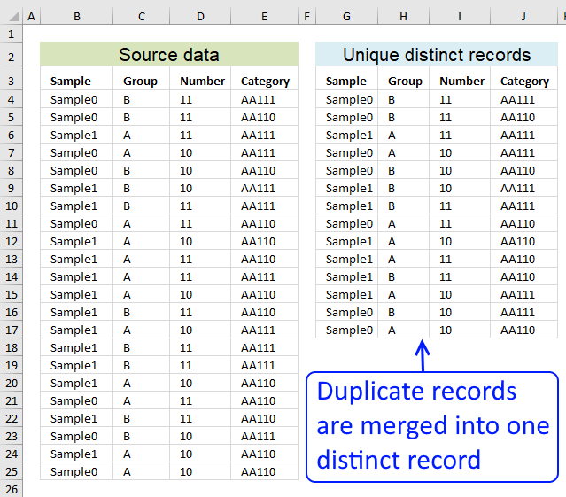
Table of contents Filter unique distinct row records Filter unique distinct row records but not blanks Filter unique distinct row […]
This article demonstrates two ways to extract unique and unique distinct rows from a given cell range. The first one […]
Excel categories
3 Responses to “Unique distinct records sorted based on count or frequency”
Leave a Reply
How to comment
How to add a formula to your comment
<code>Insert your formula here.</code>
Convert less than and larger than signs
Use html character entities instead of less than and larger than signs.
< becomes < and > becomes >
How to add VBA code to your comment
[vb 1="vbnet" language=","]
Put your VBA code here.
[/vb]
How to add a picture to your comment:
Upload picture to postimage.org or imgur
Paste image link to your comment.
Thi site helped me crate a list of unique users from a data extract however I want to go one more step and next o the unique user add in the location they are at. Location is column A, user is column B and unique user is in column I, in column J I just want to have their location - can you direct or guide me to the tip to clip? Thank you!!
William J. Ryan,
Formula in J2:
Great formula! However, my list contains blank values. How do I account for this? With the above formula, the last value is repeated.