Filter unique distinct records case sensitive

This article demonstrates two ways to extract unique and unique distinct rows from a given cell range. The first one is an Excel 365 LAMBDA function, the second is a User Defined Function.
Table of contents
1. Introduction
What are unique values?
A value refers to the contents of a single cell in a spreadsheet or data set. A unique value is a value that appears only once in the entire data set.
What are unique rows?
A row is a horizontal set of values across multiple columns in a dataset. A unique row is a row that appears only once in the dataset. If two or more rows have the exact same values across all columns they are not unique.
What are unique distinct rows?
A unique distinct row means that duplicate rows in a dataset are removed, leaving only one instance of each distinct row. In other words, if multiple rows have identical values across all columns, they are merged into a single row in the final dataset. This process ensures that each row is unique, with no duplicates.
What is an Excel 365 dynamic array formula?
A dynamic array formula in Excel 365 automatically spills results into multiple cells without needing to copy the formula manually. You only need to press Enter after typing an Excel 365 formula in contrast to array formulas in older Excel versions where you had to enter the formula by pressing CTRL + SHIFT + Enter and then copy the formula to adjacent cells in order to display all values in the returning array.
What is a LAMBDA function?
The LAMBDA function in Excel allows users to create custom, reusable functions without VBA. It enables defining a formula with named parameters making it easier to simplify complex calculations and reuse logic across a workbook.
What is a User Defined Function (UDF)?
A User Defined Function (UDF) is a custom function created using VBA (Visual Basic for Applications) in Excel to perform calculations beyond built-in functions. UDFs extend Excel’s capabilities and can be used just like standard formulas and array formulas.
What is case sensitive?
A case-sensitive comparison distinguishes between uppercase and lowercase letters. For example, in Excel, "Apple" and "apple" are treated as different values in case-sensitive operations.
What is filtering in Excel?
Filtering in Excel allows users to display only specific rows in a dataset based on set conditions, hiding irrelevant data.
2. Filter unique rows case sensitive - Excel 365 LAMBDA function
The following formula lists unique rows from cell range B3:C8 also considering upper and lower letters, in other words, a case sensitive list. Unique rows are rows that only exist once in B3:C8.
The formula extracts row 4 and row 7, they are the only ones that are unique meaning they exist only once in the list. The other rows have at least one duplicate if you also consider upper and lower letters.
Excel 365 formula in cell E3:
The formula works only in Excel 365, it uses the FILTER, BYROW, and LAMBDA functions which are only available in Excel 365. It spills values to cells below and to the right as far as needed. A #SPILL! error means that the destination cells are not empty, find the populated cells and delete or remove the values.
Explaining formula
Step 1 - Case sensitive compare
The EXACT function checks if two values are precisely the same, it returns TRUE or FALSE. The EXACT function also considers upper case and lower case letters.
Function syntax: EXACT(text1, text2)
EXACT(a,B3:C8)
Variable a is specified in the LAMBDA function in step 10, the LAMBDA function is used together with the BYROW function to perform calculations row-wise.
For example, the first row in cell range B3:C8 is B3:C3.
EXACT(B3:C3, B3:C8)
becomes
EXACT({"A","BB"},{"A","BB";"a","BB";"A","BB";"A","bb";"a","bb";"A","bb"})
and returns
{TRUE, TRUE;FALSE, TRUE;TRUE, TRUE;TRUE, FALSE;FALSE, FALSE;TRUE, FALSE}.
Step 2 - Convert boolean to numerical
The MMULT function in step 6 requires numerical values to work properly, there are several ways to convert boolean values to their numerical equivalents. One is to use double negatives, other examples are +0 (zero), *1.
--EXACT(a,B3:C8)
becomes
--{TRUE, TRUE;FALSE, TRUE;TRUE, TRUE;TRUE, FALSE;FALSE, FALSE;TRUE, FALSE}
and returns
{1, 1;0, 1;1, 1;1, 0;0, 0;1, 0}.
Step 3 - Calculate column numbers in given cell range
The COLUMN function returns the column number of the top-left cell of a cell reference.
Function syntax: COLUMN(reference)
COLUMN(B3:C8)
returns
{2, 3}
Step 4 - Raise array to the power of 0 (zero)
The ^ caret character represents an exponent, in this case, an array raised to the power of 0 (zero). This creates an array containing only 1's.
COLUMN(B3:C8)^0
becomes
{2, 3}^0
and returns
{1, 1}
Step 5 - Rearrange values from horizontal to vertical
The TRANSPOSE function converts a vertical range to a horizontal range, or vice versa.
Function syntax: TRANSPOSE(array)
TRANSPOSE(COLUMN(B3:C8)^0)
becomes
TRANSPOSE({1, 1})
and returns
{1; 1}
Step 6 - Perform matrix multiplication
The MMULT function calculates the matrix product of two arrays, an array as the same number of rows as array1 and columns as array2.
Function syntax: MMULT(array1, array2)
MMULT(--EXACT(a,B3:C8),TRANSPOSE(COLUMN(B3:C8)^0))
The following calculation is only for the first row, the formula calculates the remaining rows as well but not shown here.
MMULT(--EXACT(B3:C3,B3:C8),TRANSPOSE(COLUMN(B3:C8)^0))
becomes
MMULT({1,1;0,1;1,1;1,0;0,0;1,0},{1;1})
and returns
{2; 1; 2; 1; 0; 1}.
Step 7 - Check if numbers are larger than 1
The larger than character is a logical operator, it lets you check if a value is larger than another given value. The result is a boolean value TRUE or FALSE.
MMULT(--EXACT(a,B3:C8),TRANSPOSE(COLUMN(B3:C8)^0))>1
becomes
{2; 1; 2; 1; 0; 1}>1
and returns
{TRUE; FALSE; TRUE; FALSE; FALSE; FALSE}
Step 8 - Convert boolean to numerical
The SUM function can't process boolean values, we must once again convert the boolean values to their numerical equivalents using double negatives just like in step 2.
--(MMULT(--EXACT(a,B3:C8),TRANSPOSE(COLUMN(B3:C8)^0))>1)
becomes
--(MMULT(--EXACT(B3:C3,B3:C8),TRANSPOSE(COLUMN(B3:C8)^0))>1)
becomes
--{TRUE; FALSE; TRUE; FALSE; FALSE; FALSE}
and returns
{1; 0; 1; 0; 0; 0}.
This array tells us that the value in cell B3:C3 (first position in the array) is exactly the same as the value in the third position in the array. The position in the array corresponds to the position in cell range B3:C8.
Step 9 - Add numbers and return a total
The SUM function allows you to add numerical values, the function returns the sum in the cell it is entered in. The SUM function is cleverly designed to ignore text and boolean values, adding only numbers.
Function syntax: SUM(number1, [number2], ...)
SUM(--(MMULT(--EXACT(a,B3:C8),TRANSPOSE(COLUMN(B3:C8)^0))>1))
becomes
SUM({1; 0; 1; 0; 0; 0})
and returns 2. This means that the first row has a duplicate and its located on row 3. Number 1 in the array is also in the third position.
Step 10 - Build LAMBDA function
The LAMBDA function build custom functions without VBA, macros or javascript.
Function syntax: LAMBDA([parameter1, parameter2, …,] calculation)
LAMBDA(a,SUM(--(MMULT(--EXACT(a,B3:C8),TRANSPOSE(COLUMN(B3:C8)^0))>1)))
The LAMBDA function is needed for the BYROW function to work properly.
Step 11 - Perform calculations row-wise
The BYROW function puts values from an array into a LAMBDA function row-wise.
Function syntax: BYROW(array, lambda(array, calculation))
BYROW(B3:C8,LAMBDA(a,SUM(--(MMULT(--EXACT(a,B3:C8),TRANSPOSE(COLUMN(B3:C8)^0))>1))))
Step 12 - Filter rows if array is equal to 1
The FILTER function extracts values/rows based on a condition or criteria.
Function syntax: FILTER(array, include, [if_empty])
FILTER(B3:C8,BYROW(B3:C8,LAMBDA(a,SUM(--(MMULT(--EXACT(a,B3:C8),TRANSPOSE(COLUMN(B3:C8)^0))>1))))=1)
becomes
FILTER(B3:C8,{2;1;2;2;1;2}=1)
becomes
FILTER(B3:C8,{FALSE;TRUE;FALSE;FALSE;TRUE;FALSE})
and returns
{"a", "BB"; "a", "bb"}.
3. Count unique rows case sensitive - Excel 365 LAMBDA function

This formula displayed in the image above counts unique rows also considering upper and lower letters whereas the formula in section 2 lists unique rows. The image above demonstrates an Excel 365 formula in cell F3 that calculates the number of unique rows but also considering upper and lower letters, specified in cell range C3:D8.
Excel 365 LAMBDA formula in cell F3:
The unique rows are in B4:C4 and B7:C7, the remaining rows have at least one duplicate and is therefore not unique. The formula returns 2 which represents two unique rows in cells B3:C8. The formula works only in Excel 365, it uses the BYROW, and LAMBDA functions which are only available in Excel 365. It returns only one value which represents the number of unique rows in cells B3:C8.
Replace all instances of B3:C8 in the formula above with a cell reference that points to cell range you want to use as source data. That is all you need to do in order to use the formula.
Explaining formula
Step 1 - Case sensitive compare
The EXACT function checks if two values are precisely the same, it returns TRUE or FALSE. The EXACT function also considers upper case and lower case letters.
Function syntax: EXACT(text1, text2)
EXACT(a,B3:C8)
Variable a is specified in the LAMBDA function in step 10, the LAMBDA function is used together with the BYROW function to perform calculations row-wise.
For example, the first row in cell range B3:C8 is B3:C3.
EXACT(B3:C3, B3:C8)
becomes
EXACT({"A","BB"},{"A","BB";"a","BB";"A","BB";"A","bb";"a","bb";"A","bb"})
and returns
{TRUE, TRUE;FALSE, TRUE;TRUE, TRUE;TRUE, FALSE;FALSE, FALSE;TRUE, FALSE}.
Step 2 - Convert boolean to numerical
The MMULT function in step 6 requires numerical values to work properly, there are several ways to convert boolean values to their numerical equivalents. One is to use double negatives, other examples are +0 (zero), *1.
--EXACT(a,B3:C8)
becomes
--{TRUE, TRUE;FALSE, TRUE;TRUE, TRUE;TRUE, FALSE;FALSE, FALSE;TRUE, FALSE}
and returns
{1, 1;0, 1;1, 1;1, 0;0, 0;1, 0}.
Step 3 - Calculate column numbers in given cell range
The COLUMN function returns the column number of the top-left cell of a cell reference.
Function syntax: COLUMN(reference)
COLUMN(B3:C8)
returns
{2, 3}
Step 4 - Raise array to the power of 0 (zero)
The ^ caret character represents an exponent, in this case, an array raised to the power of 0 (zero). This creates an array containing only 1's.
COLUMN(B3:C8)^0
becomes
{2, 3}^0
and returns
{1, 1}
Step 5 - Rearrange values from horizontal to vertical
The TRANSPOSE function converts a vertical range to a horizontal range, or vice versa.
Function syntax: TRANSPOSE(array)
TRANSPOSE(COLUMN(B3:C8)^0)
becomes
TRANSPOSE({1, 1})
and returns
{1; 1}
Step 6 - Perform matrix multiplication
The MMULT function calculates the matrix product of two arrays, an array as the same number of rows as array1 and columns as array2.
Function syntax: MMULT(array1, array2)
MMULT(--EXACT(a,B3:C8),TRANSPOSE(COLUMN(B3:C8)^0))
The following calculation is only for the first row, the formula calculates the remaining rows as well but not shown here.
MMULT(--EXACT(B3:C3,B3:C8),TRANSPOSE(COLUMN(B3:C8)^0))
becomes
MMULT({1,1;0,1;1,1;1,0;0,0;1,0},{1;1})
and returns
{2; 1; 2; 1; 0; 1}.
Step 7 - Check if numbers are larger than 1
The larger than character is a logical operator, it lets you check if a value is larger than another given value. The result is a boolean value TRUE or FALSE.
MMULT(--EXACT(a,B3:C8),TRANSPOSE(COLUMN(B3:C8)^0))>1
becomes
{2; 1; 2; 1; 0; 1}>1
and returns
{TRUE; FALSE; TRUE; FALSE; FALSE; FALSE}.
Remember that the above array calculation is only for B3:C3, the remaining rows will also be calculated , however, not shown here.
Step 8 - Convert boolean to numerical
The SUM function can't process boolean values, we must once again convert the boolean values to their numerical equivalents using double negatives just like in step 2.
--(MMULT(--EXACT(a,B3:C8),TRANSPOSE(COLUMN(B3:C8)^0))>1)
becomes
--(MMULT(--EXACT(B3:C3,B3:C8),TRANSPOSE(COLUMN(B3:C8)^0))>1)
becomes
--{TRUE;FALSE;TRUE;FALSE;FALSE;FALSE}
and returns
{1; 0; 1; 0; 0; 0}.
This array tells us that the value in cell B3:C3 (first position in the array) is exactly the same as the value in the third position in the array. The position in the array corresponds to the position in cell range B3:C8.
Step 9 - Add numbers and return a total
The SUM function allows you to add numerical values, the function returns the sum in the cell it is entered in. The SUM function is cleverly designed to ignore text and boolean values, adding only numbers.
Function syntax: SUM(number1, [number2], ...)
SUM(--(MMULT(--EXACT(a,B3:C8),TRANSPOSE(COLUMN(B3:C8)^0))=1))
becomes
SUM({1; 0; 1; 0; 0; 0})
and returns 2. This means that the first row has a duplicate and its located on row 3. Number 1 in the array is also in the third position.
Step 10 - Build LAMBDA function
The LAMBDA function build custom functions without VBA, macros or javascript.
Function syntax: LAMBDA([parameter1, parameter2, …,] calculation)
LAMBDA(a,SUM(--(MMULT(--EXACT(a,B3:C8),TRANSPOSE(COLUMN(B3:C8)^0))=1)))
The LAMBDA function is needed for the BYROW function to work properly.
Step 11 - Perform calculations row-wise
The BYROW function puts values from an array into a LAMBDA function row-wise.
Function syntax: BYROW(array, lambda(array, calculation))
BYROW(B3:C8,LAMBDA(a,SUM(--(MMULT(--EXACT(a,B3:C8),TRANSPOSE(COLUMN(B3:C8)^0))=1))))
returns
{2; 1; 2; 2; 1; 2}.
This array shows the calculation for each row. B3:C3 is the first row, it returned 2 which is the first value in the array. B4:C4 returns 1 which is the second value in the array, and so on.
Step 12 - Compare with 1
The equal sign lets you compare values in an Excel formula, it is a logical operator and returns TRUE or FALSE. By comparing the array with 1 we can celculate the number of unique rows there is in cell range B3:C8.
--(BYROW(B3:C8,LAMBDA(a,SUM(--(MMULT(--EXACT(a,B3:C8),TRANSPOSE(COLUMN(B3:C8)^0))>1))))=1)
becomes
--({2; 1; 2; 2; 1; 2}=1)
becomes
--({FALSE; TRUE; FALSE; FALSE; TRUE; FALSE})
and returns
{0; 1; 0; 0; 1; 0}.
Step 13 - Add numbers and return total
The SUM function allows you to add numerical values, the function returns the sum in the cell it is entered in. The SUM function is cleverly designed to ignore text and boolean values, adding only numbers.
Function syntax: SUM(number1, [number2], ...)
SUM(--(BYROW(B3:C8,LAMBDA(a,SUM(--(MMULT(--EXACT(a,B3:C8),TRANSPOSE(COLUMN(B3:C8)^0))>1))))=1))
becomes
SUM({0; 1; 0; 0; 1; 0})
and returns 2. There are two unique rows, also considering upper and lower letters, in cell range C3:D8.
4. Filter unique distinct rows case sensitive - Excel 365 recursive LAMBDA function

The following formula extracts unique distinct rows, also considering upper and lower letters, from a given cell range. The formula is dynamic meaning it takes into account the number of columns as well. This means that the formula also works for cell ranges larger than two columns.
If your cell range only has one column then use this much smaller formula: Extract a case sensitive unique list from a column - Excel 365
How to use the formula? Change cell reference B3:C8 to your needs, there are two instances of B3:C8 that need to be changed in the formula below.
Excel 365 recursive LAMBDA formula in cell E3:
IF(n=(ROWS(rng)+1),DROP(result,1),
IF(SUM(--(MMULT(--EXACT(INDEX(rng,n,0),result),TRANSPOSE(COLUMN(rng)^0))=COLUMNS(rng))),
ME(ME,rng,n+1,result),ME(ME,rng,n+1,VSTACK(result,INDEX(rng,n,0))))))
,UDRCS(UDRCS,B3:C8,1,EXPAND("",1,COLUMNS(B3:C8),"")))
The formula works only in Excel 365, it uses the LET, EXPAND, VSTACK and LAMBDA functions which are only available in Excel 365. It returns only one value which represents the number of unique rows in cells B3:C8.
This formula defines a recursive LAMBDA function named UDRCS that iterates through each row of the specified range (rng). It checks if the current row is already present in the accumulated result. If not, it adds the row to result. The recursion continues until all rows are processed, resulting in a collection of unique distinct rows with duplicate rows removed.
What is a recursive function?
In Excel, a recursive function is one that calls itself to solve a problem by breaking it down into smaller more manageable sub-problems. With the introduction of the LAMBDA function,Excel now supports the creation of such recursive functions directly within worksheets. This removes the need for VBA macros in some cases.
Explaining formula
Step 1 - Get n-th row from array rng
The INDEX function returns a value or reference from a cell range or array, you specify which value based on a row and column number.
Function syntax: INDEX(array, [row_num], [column_num])
INDEX(rng,n,0)
Step 2 - Check if values in row match the result array
The EXACT function checks if two values are precisely the same, it returns TRUE or FALSE. The EXACT function also considers upper case and lower case letters.
Function syntax: EXACT(text1, text2)
EXACT(INDEX(rng,n,0),result)
Step 3 - Convert boolean values to numerical values
--EXACT(INDEX(rng,n,0),result)
Step 4 - Create column numbers based on rng
The COLUMN function returns the column number of the top-left cell of a cell reference.
Function syntax: COLUMN(reference)
COLUMN(rng)
Step 5 - Replace numbers with 1's
COLUMN(rng)^0
Step 6 - Rearrange values from horizontal to vertical layout
The TRANSPOSE function converts a vertical range to a horizontal range, or vice versa.
Function syntax: TRANSPOSE(array)
TRANSPOSE(COLUMN(rng)^0))
Step 7 -
The MMULT function calculates the matrix product of two arrays, an array as the same number of rows as array1 and columns as array2.
Function syntax: MMULT(array1, array2)
MMULT(--EXACT(INDEX(rng,n,0),result),TRANSPOSE(COLUMN(rng)^0)
Step 8 - Convert boolean values to numerical values
--(MMULT(--EXACT(INDEX(rng,n,0),result),TRANSPOSE(COLUMN(rng)^0)
Step 9 - Add numerical values and return a total
The SUM function allows you to add numerical values, the function returns the sum in the cell it is entered in. The SUM function is cleverly designed to ignore text and boolean values, adding only numbers.
Function syntax: SUM(number1, [number2], ...)
SUM(--(MMULT(--EXACT(INDEX(rng,n,0),result),TRANSPOSE(COLUMN(rng)^0))
Step 10 - Check if row values exist in result variable
The IF function returns one value if the logical test is TRUE and another value if the logical test is FALSE.
Function syntax: IF(logical_test, [value_if_true], [value_if_false])
IF(SUM(--(MMULT(--EXACT(INDEX(rng,n,0),result),TRANSPOSE(COLUMN(rng)^0))=COLUMNS(rng))),
ME(ME,rng,n+1,result),ME(ME,rng,n+1,VSTACK(result,INDEX(rng,n,0)))))
Step 11 - Control recursive function
The DROP function removes a given number of rows or columns from a 2D cell range or array.
Function syntax: DROP(array, rows, [columns])
IF(n=(ROWS(rng)+1),DROP(result,1),
IF(SUM(--(MMULT(--EXACT(INDEX(rng,n,0),result),TRANSPOSE(COLUMN(rng)^0))=COLUMNS(rng))),
ME(ME,rng,n+1,result),ME(ME,rng,n+1,VSTACK(result,INDEX(rng,n,0))))))
Step 12 - Build LAMBDA function
The LAMBDA function build custom functions without VBA, macros or javascript.
Function syntax: LAMBDA([parameter1, parameter2, …,] calculation)
LAMBDA(ME,rng,n,result,
IF(n=(ROWS(rng)+1),DROP(result,1),
IF(SUM(--(MMULT(--EXACT(INDEX(rng,n,0),result),TRANSPOSE(COLUMN(rng)^0))=COLUMNS(rng))),
ME(ME,rng,n+1,result),ME(ME,rng,n+1,VSTACK(result,INDEX(rng,n,0))))))
Step 13 - Name LAMBDA function and populate variables
The LET function lets you name intermediate calculation results which can shorten formulas considerably and improve performance.
Function syntax: LET(name1, name_value1, calculation_or_name2, [name_value2, calculation_or_name3...])
LET(UDRCS,LAMBDA(ME,rng,n,result,
IF(n=(ROWS(rng)+1),DROP(result,1),
IF(SUM(--(MMULT(--EXACT(INDEX(rng,n,0),result),TRANSPOSE(COLUMN(rng)^0))=COLUMNS(rng))),
ME(ME,rng,n+1,result),ME(ME,rng,n+1,VSTACK(result,INDEX(rng,n,0))))))
,UDRCS(UDRCS,B3:C8,1,EXPAND("",1,COLUMNS(B3:C8),"")))
5. Count unique distinct rows case sensitive - Excel 365 LAMBDA function

The Excel 365 formula in cell F3 shown in the image above calculates the number of unqiue distinct rows, also considering upper and lower letters, specified in cell range C3:D8.
I have bolded, and put numbers next to, unique distinct rows in the image above.
Excel 365 LAMBDA formula in cell F3:
Explaining formula
Step 1 - Case sensitive compare
The EXACT function checks if two values are precisely the same, it returns TRUE or FALSE. The EXACT function also considers upper case and lower case letters.
Function syntax: EXACT(text1, text2)
EXACT(a,B3:C8)
Variable a is specified in the LAMBDA function in step 10, the LAMBDA function is used together with the BYROW function to perform calculations row-wise.
For example, the first row in cell range B3:C8 is B3:C3.
EXACT(B3:C3, B3:C8)
becomes
EXACT({"A","BB"},{"A","BB";"a","BB";"A","BB";"A","bb";"a","bb";"A","bb"})
and returns
{TRUE, TRUE;FALSE, TRUE;TRUE, TRUE;TRUE, FALSE;FALSE, FALSE;TRUE, FALSE}.
Step 2 - Convert boolean to numerical
The MMULT function in step 6 requires numerical values to work properly, there are several ways to convert boolean values to their numerical equivalents. One is to use double negatives, other examples are +0 (zero), *1.
--EXACT(a,B3:C8)
becomes
--{TRUE, TRUE;FALSE, TRUE;TRUE, TRUE;TRUE, FALSE;FALSE, FALSE;TRUE, FALSE}
and returns
{1, 1;0, 1;1, 1;1, 0;0, 0;1, 0}.
Step 3 - Calculate column numbers in given cell range
The COLUMN function returns the column number of the top-left cell of a cell reference.
Function syntax: COLUMN(reference)
COLUMN(B3:C8)
returns
{2, 3}
Step 4 - Raise array to the power of 0 (zero)
The ^ caret character represents an exponent, in this case, an array raised to the power of 0 (zero). This creates an array containing only 1's.
COLUMN(B3:C8)^0
becomes
{2, 3}^0
and returns
{1, 1}
Step 5 - Rearrange values from horizontal to vertical
The TRANSPOSE function converts a vertical range to a horizontal range, or vice versa.
Function syntax: TRANSPOSE(array)
TRANSPOSE(COLUMN(B3:C8)^0)
becomes
TRANSPOSE({1, 1})
and returns
{1; 1}
Step 6 - Perform matrix multiplication
The MMULT function calculates the matrix product of two arrays, an array as the same number of rows as array1 and columns as array2.
Function syntax: MMULT(array1, array2)
MMULT(--EXACT(a,B3:C8),TRANSPOSE(COLUMN(B3:C8)^0))
The following calculation is only for the first row, the formula calculates the remaining rows as well but not shown here.
MMULT(--EXACT(B3:C3,B3:C8),TRANSPOSE(COLUMN(B3:C8)^0))
becomes
MMULT({1,1;0,1;1,1;1,0;0,0;1,0},{1;1})
and returns
{2; 1; 2; 1; 0; 1}.
Step 7 - Check if numbers are larger than 1
The larger than character is a logical operator, it lets you check if a value is larger than another given value. The result is a boolean value TRUE or FALSE.
MMULT(--EXACT(a,B3:C8),TRANSPOSE(COLUMN(B3:C8)^0))>1
becomes
{2; 1; 2; 1; 0; 1}>1
and returns
{TRUE; FALSE; TRUE; FALSE; FALSE; FALSE}
Step 8 - Convert boolean to numerical
The SUM function can't process boolean values, we must once again convert the boolean values to their numerical equivalents using double negatives just like in step 2.
--(MMULT(--EXACT(a,B3:C8),TRANSPOSE(COLUMN(B3:C8)^0))>1)
becomes
--(MMULT(--EXACT(B3:C3,B3:C8),TRANSPOSE(COLUMN(B3:C8)^0))>1)
becomes
--{TRUE; FALSE; TRUE; FALSE; FALSE; FALSE}
and returns
{1; 0; 1; 0; 0; 0}.
This array tells us that the value in cell B3:C3 (first position in the array) is exactly the same as the value in the third position in the array. The position in the array corresponds to the position in cell range B3:C8.
Step 9 - Add numbers and return a total
The SUM function allows you to add numerical values, the function returns the sum in the cell it is entered in. The SUM function is cleverly designed to ignore text and boolean values, adding only numbers.
Function syntax: SUM(number1, [number2], ...)
SUM(--(MMULT(--EXACT(a,B3:C8),TRANSPOSE(COLUMN(B3:C8)^0))>1))
becomes
SUM({1; 0; 1; 0; 0; 0})
and returns 2. This means that the first row has a duplicate and its located on row 3. Number 1 in the array is also in the third position.
Step 10 - Build LAMBDA function
The LAMBDA function build custom functions without VBA, macros or javascript.
Function syntax: LAMBDA([parameter1, parameter2, …,] calculation)
LAMBDA(a,SUM(--(MMULT(--EXACT(a,B3:C8),TRANSPOSE(COLUMN(B3:C8)^0))>1)))
The LAMBDA function is needed for the BYROW function to work properly.
Step 11 - Perform calculations row-wise
The BYROW function puts values from an array into a LAMBDA function row-wise.
Function syntax: BYROW(array, lambda(array, calculation))
BYROW(B3:C8,LAMBDA(a,SUM(--(MMULT(--EXACT(a,B3:C8),TRANSPOSE(COLUMN(B3:C8)^0))>1))))
Step 12 - Divide 1 by all numbers in the array
The division character lets you dived numbers in an Excel formula.
1/BYROW(C3:D8,LAMBDA(a,SUM(--(MMULT(--EXACT(a,C3:D8),TRANSPOSE(COLUMN(C3:D8)^0))>1))))
becomes
1/{2; 1; 2; 2; 1; 2}
and returns
{0.5; 1; 0.5; 0.5; 1; 0.5}.
Step 13 - Add numbers and return total
The SUM function allows you to add numerical values, the function returns the sum in the cell it is entered in. The SUM function is cleverly designed to ignore text and boolean values, adding only numbers.
Function syntax: SUM(number1, [number2], ...)
SUM(1/BYROW(C3:D8,LAMBDA(a,SUM(--(MMULT(--EXACT(a,C3:D8),TRANSPOSE(COLUMN(C3:D8)^0))>1)))))
becomes
SUM({0.5; 1; 0.5; 0.5; 1; 0.5})
and returns 4. There are four unique distinct rows, also considering upper and lower letters, in cell range C3:D8.
6. Filter unique distinct records case sensitive - UDF
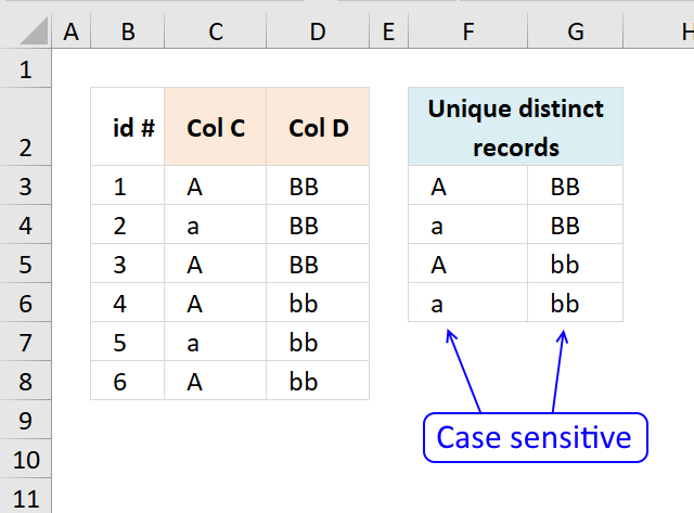
The User Defined Function demonstrated above extracts unique distinct records also considering upper and lower case letters. For example, a record containing A and B is not the same as a record containing a and b.
A User defined Function is a custom function anyone can build, you simply add the VBA code to your workbook and you are good to go.
Array formula in cell F3:G6:
The formula returns unique distinct rows based on upper and lower letters. The custom built formula uses VBA code to accomplish the output which is different to regular formulas that uses built-in functions.
Note! The following steps are only needed in older Excel versions, Excel 365 users can skip these steps.
To enter an array formula:
- Type the formula in a cell
- Press and hold CTRL + SHIFT simultaneously
- Press Enter once.
- Release all keys.
The formula bar now shows the formula with a beginning and ending curly bracket telling you that you entered the formula successfully. Don't enter the curly brackets yourself.
6.1 User defined Function Syntax
UniqueRecords(rng)
6.2 Arguments
| Parameter | Text |
| rng | Required. The range you want to use. |
6.3 Where to copy VBA code?
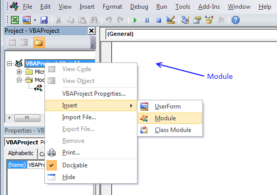
- Press Alt-F11 to open visual basic editor
- Press with left mouse button on Module on the Insert menu
- Copy and paste above vba code
- Exit visual basic editor
6.4 Excel user defined function:
'Name function and declare argument
Function UniqueRecords(rng As Variant) As Variant()
' This udf filters unique distinct records (case sensitive)
'Declare variables and data types
Dim r As Single, c As Single, temp() As Variant, k As Single
Dim rt As Single, ct As Single, a As Single, b As Single
Dim i As Single, j As Integer, iCols As Single, iRows As Single

'Save values in cell range to array variable rng (yes, same name)
rng = rng.Value
'Change size of array variable rng
ReDim temp(UBound(rng, 2) - 1, 0)
'Iterate through rows in array variable rng
For r = 1 To UBound(rng, 1)
  'Iterate through rows in array variable temp
  For rt = LBound(temp, 2) To UBound(temp, 2)
    'Iterate through columns in array variable rng
    For c = 1 To UBound(rng, 2)
      ' If temp value is equal rng value then increment variable a with 1
      If temp(c - 1, rt) = rng(r, c) Then a = a + 1
    Next c
    'If a is equal to the number of columns in rng then all values in record match
    If a = UBound(rng, 2) Then
      a = 0
      b = 0
      Exit For
    Else
      a = 0
      b = b + 1
    End If
  Next rt
  If b = UBound(temp, 2) + 1 Then
    For c = 1 To UBound(rng, 2)
      temp(c - 1, UBound(temp, 2)) = rng(r, c)
    Next c
    ReDim Preserve temp(UBound(temp, 1), UBound(temp, 2) + 1)
    b = 0
  End If
Next r

k = Range(Application.Caller.Address).Rows.Count
If Range(Application.Caller.Address).Columns.Count < UBound(rng, 2) Then
  MsgBox "There are more columns, extend user defined function to the right"
End If
If k < UBound(temp, 2) Then
  MsgBox "There are more rows, extend user defined function down"
Else
  For i = UBound(temp, 2) To k
    ReDim Preserve temp(UBound(temp, 1), i)
    For j = 0 To UBound(temp, 1)
      temp(j, i) = ""
    Next j
  Next i
End If

UniqueRecords = Application.Transpose(temp)
End Function
Unique distinct records category
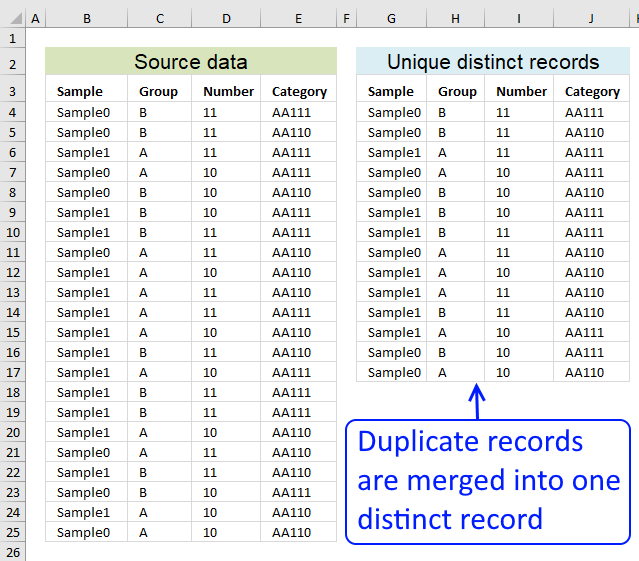
Table of contents Filter unique distinct row records Filter unique distinct row records but not blanks Filter unique distinct row […]
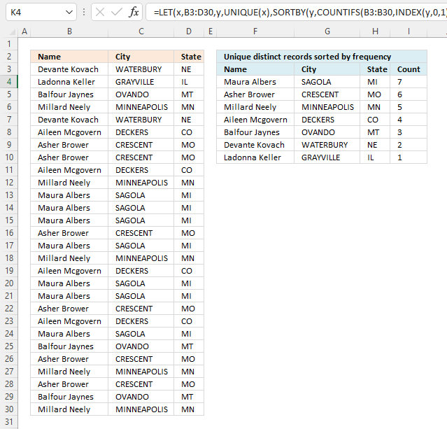
This article demonstrates how to sort records in a data set based on their count meaning the formula counts each […]
Excel categories
Leave a Reply
How to comment
How to add a formula to your comment
<code>Insert your formula here.</code>
Convert less than and larger than signs
Use html character entities instead of less than and larger than signs.
< becomes < and > becomes >
How to add VBA code to your comment
[vb 1="vbnet" language=","]
Put your VBA code here.
[/vb]
How to add a picture to your comment:
Upload picture to postimage.org or imgur
Paste image link to your comment.