Excel calendar
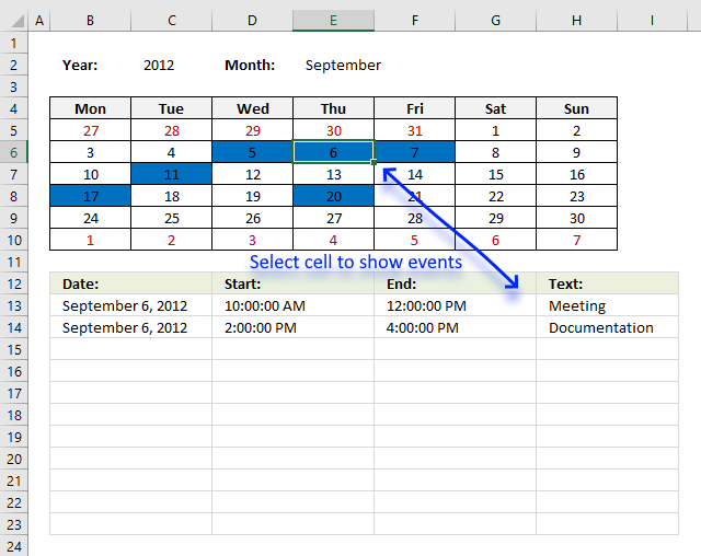
Table of Contents
- Excel monthly calendar - VBA
- Calendar
- Conditional formatting
- Formulas
- Visual basic for applications
- Get excel *.xlsm file
- Excel weekly calendar with scheduling - VBA
- Get Excel *.xlsm file
- Weekly schedule template
- Setting up your work hours in a weekly schedule
- Highlight specific time ranges in a weekly schedule
- Weekly appointment calendar
- Schedule recurring expenses in a calendar
- Count groups in calendar
- Free School Schedule Template
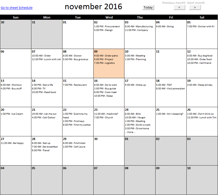
1. Excel monthly calendar - VBA
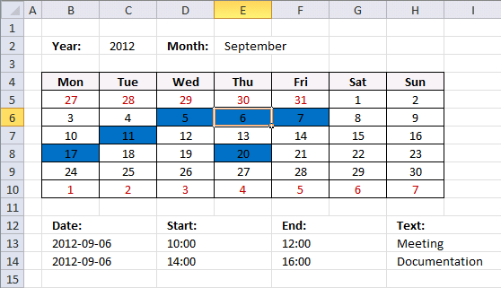
This workbook contains two worksheets, one worksheet shows a calendar and the other worksheet is used to store events. The calendar sheet allows you to enter a year and use a drop down list to select a month.
A small VBA event code tracks which cell you have selected and shows the corresponding events accordingly.
How this workbook works

The animated image above shows how to enter data and how to select a given date. Today's date is highlighted yellow, days with one or more events are also highlighted, in this example blue.
Excel extracts data dynamically meaning the named range grows automatically when new data is entered, we don't need to change the formula cell references.
Drop down lists
Select year
- Select cell B2
- Go to tab "Data"
- Press with left mouse button on "Data Validation" button

- Allow: List
- Source:2012,2013,2014,2015,2016
- Press with left mouse button on OK
Select month
- Select cell E4
- Go to tab "Data"
- Press with left mouse button on "Data Validation" button
- Allow: List
- Source:January, February, March, April, May, June, July, August, September, October, November, December
- Press with left mouse button on OK
Headers

Type Year: in cell B2, Month: in cell E2 and so on...
Calculating dates (formula)
- Select cell B5
- Formula:
=DATE($C$2,MATCH($E$2,{"January"; "February"; "March"; "April"; "May"; "June"; "July"; "August"; "September"; "October"; "November"; "December"},0),1)-WEEKDAY(DATE($C$2,MATCH($E$2,{"January"; "February"; "March"; "April"; "May"; "June"; "July"; "August"; "September"; "October"; "November"; "December"},0),1),2)+1
- Select cell B6
- Formula:
=B5+1
- Copy cell B6 (Ctrl + c)
- Select cell range D5:H5
- Paste (Ctrl + v)
- Select cell B6
- Formula:
=B5+7
- Copy cell range C5:H5
- Select cell range C6:H6
- Paste (Ctrl + v)
- Copy cell range B6:H6 (Ctrl + c)
- Select cell range B7:H10
- Paste (Ctrl + v)
Conditional formatting
Highlight Today
- Select cell range B5:H10

- Go to tab "Home"
- Press with left mouse button on "Conditional formatting" button
- Press with left mouse button on "New Rule..."
- Press with left mouse button on "Use a formula to determine which cells to format"
- Format values where this formula is true:
=B5=TODAY() - Press with left mouse button on "Format..." button
- Go to "Fill" tab
- Pick a color
- Press with left mouse button on OK
- Press with left mouse button on OK
Change font color for dates not in selected month
- Repeat 1-5 steps above
- =MONTH(B5)<>MONTH($B$6)
- Press with left mouse button on "Format..." button
- Go to "Font" tab
- Pick a color
- Press with left mouse button on OK
- Press with left mouse button on OK
Highlight days with events
- Repeat 1-5 steps above
- =OR(B5=INT(INDEX(Data,0,1)))
- Press with left mouse button on "Format..." button
- Go to "Fill" tab
- Pick a color
- Press with left mouse button on OK
- Press with left mouse button on OK
Formulas
Dynamic named range
- Select sheet "Data"
- Go to tab "Formulas"
- Press with left mouse button on "Name Manager" button
- Press with left mouse button on "New..."

- Name: Data
- Refers to:
=OFFSET(Data!$A$2,,,COUNTA(Data!$A$1:$A$1000)-1,3) - Press with left mouse button on OK!
- Press with left mouse button on Close
Event formulas
- Select sheet "Calendar"
- Select cell B13

- Array formula:
=IFERROR(INT(INDEX(Data, SMALL(IF(INT(INDEX(Data, 0, 1))=$G$2, MATCH(ROW(Data), ROW(Data)), ""), ROW(A1)), COLUMN(A1))), "")
- Enter this formula as an array formula, see these steps if you don't know how.
- Select cell D13
- Array formula:
=IFERROR(INDEX(Data, SMALL(IF(INT(INDEX(Data, 0, 1))=$G$2, MATCH(ROW(Data), ROW(Data)), ""), ROW(B1)), COLUMN(A1)), "")
- Select cell F13
- Array formula:
=IFERROR(INDEX(Data, SMALL(IF(INT(INDEX(Data, 0, 1))=$G$2, MATCH(ROW(Data), ROW(Data)), ""), ROW(C1)), COLUMN(B1)), "")
- Select cell H13
- Array formula:
=IFERROR(INDEX(Data, SMALL(IF(INT(INDEX(Data, 0, 1))=$G$2, MATCH(ROW(Data), ROW(Data)), ""), ROW(D1)), COLUMN(C1)), "")
How to create an array formula
- Select a cell
- Press with left mouse button on in formula bar

- Paste array formula
- Press and hold Ctrl + Shift
- Press Enter
Visual basic for applications
- Press with right mouse button on on Calendar sheet
- Press with left mouse button on "View code"
- Copy vba code below.
'Event code that is rund every time a cell is selected in worksheet Calendar Private Sub Worksheet_SelectionChange(ByVal Target As Range) 'Check if selected cell address is in cell range B5:H10 If Not Intersect(Target, Range("B5:H10")) Is Nothing Then 'Save date to cell G2 Range("G2") = Target.Value End If End Sub - Paste to worksheet module.

Hide value in cell G2
- Select cell G2
- Press Ctrl + 1
- Go to tab "Number"
- Select category: Custom
- Type ;;;
- Press with left mouse button on OK!
2. Calendar with scheduling
Here is my contribution to all excel calendars out there. My calendar is created in Excel 2007 and uses both vba and formula.
I will explain how I created this calendar in an upcoming post. You can get the excel calendar file here: Excel calendar.xlsm You need to enable macros to use this calendar.

Instructions:
Select a week
- Select a week using spinner buttons or type a date in date cells
How to add a record
- Double press with left mouse button on a cell
- Type text in title window and text window
- Press with left mouse button on Save button on userform
How to delete a record
- Double press with left mouse button on a cell
- Press with left mouse button on Delete button on userform

Overview Calendar

The overview calendar makes spinner button navigation easier. The selected week is colored gray and the date today is yellow.
3. Weekly schedule template
I would like to share this simple weekly schedule I created.
How to use weekly schedule
- Type any date in cell F2 and press Enter.
Now what?
All dates in chosen week are dynamically updated. See cell range C4:I4.
Why?
You can easily create and print multiple weekly schedules quickly without editing each date in week.
Monthly calendars
If you are looking for a monthly calendars, this might be of interest:
Get excel template
Create a weekly schedule.xls
(Excel 97-2003 Workbook *.xls)
Formula in C4:
Formula in D4:
Added features
- How to highlight specific time ranges
- How to find empty hours
- How to populate cells dynamically
- Setting up your work hours
- Schedule recurring events in a weekly schedule in excel
4. Setting up your work hours in a weekly schedule

The image above demonstrates conditional formatting highlighting hours outside work hours, those cells are filled with grey except weekends.
Conditional formatting formula applied on cell range C6:I29:
This formula checks if the weekday in C4:I4 is 2,3,4,5 or 6. (Monday to Friday) and if the time in cell range B6:B29 is outside workhours specified in cell C31 and C32. If formula returns TRUE, the cell is filled grey.
Explaining conditional formatting in cell C9
Step 1 - Check if time $B6 is less than start hour $C$31
$B6<$C$31
returns TRUE.
Step 2 - Check if time $B6 is larger than or equal to start hour $C$32
$B6>=$C$32
returns FALSE
Step 3 - If any of the logical expressions evaluate to TRUE then return TRUE
The OR function checks whether any of the arguments are TRUE or FALSE and returns FALSE if all arguments are FALSE.
OR($B6<$C$31, $B6>=$C$32)
becomes
OR(TRUE, FALSE)
and returns TRUE.
Step 4 - Check if weekday is less than 7 (Saturday)
The WEEKDAY function returns a number from 1 to 7 identifying the day of the week of a date.
WEEKDAY(C$4)<7
becomes
WEEKDAY(40391)<7
and returns TRUE.
Step 5 - Check if weekday number is larger than 1 (Sunday)
WEEKDAY(C$4)>1
becomes
WEEKDAY(40391)<1
and returns FALSE.
Step 6 - Both logical expressions must be TRUE
The AND function checks whether all arguments are TRUE and returns TRUE if all arguments are TRUE.
AND(WEEKDAY(C$4)<7, WEEKDAY(C$4)>1)
becomes
AND(TRUE, FALSE)
and returns FALSE.
Step 7 - AND logic
AND(OR($B6<$C$31, $B6>=$C$32), AND(WEEKDAY(C$4)<7, WEEKDAY(C$4)>1))
becomes
AND(TRUE, FALSE)
and returns FALSE. Cell C6 is not highlighted.
5. Highlight specific time ranges in a weekly schedule

In a previous post I created a simple weekly schedule with dynamic dates, in this post I am going to highlight hours using date and time ranges, demonstrated in the picture above Here are some random date and time ranges:

Try change date in cell F2 and see how any other week has no highlighted cells (hours).
How to highlight cells in a weekly schedule (conditional formatting)
Conditional formatting does not accept cell references outside current worksheet.
But there is a workaround.
Create a named range for each column and use the named ranges in a conditional formatting formula.
Create named ranges
- Select sheet "Time ranges"
- Select range B3:B5
- Type "Start" in name boxand press Enter

- Select range C3:C5
- Type "End" in name box and press Enter
Create conditional formatting (Excel 2007)
- Select sheet "Weekly schedule"
- Select cell range C6:I30
- Press with left mouse button on "Home" tab on the ribbon
- Press with left mouse button on "Conditional formatting"
- Press with left mouse button on "New Rule.."
- Press with left mouse button on "Use a formula to determine which cells to format"
- Type in "Format values where this formula is true" window:
=SUMPRODUCT((C6>=Start)*(C6<End)) - Press with left mouse button on "Format..." button
- Select "Fill" tab
- Select a color
- Press with left mouse button on Ok
- Press with left mouse button on Ok
- Press with left mouse button on Ok
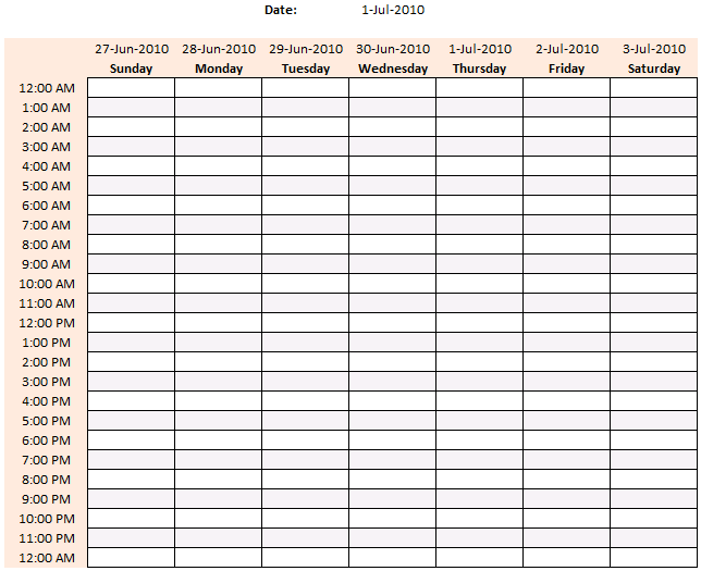
6. Weekly appointment calendar

This weekly calendar is easy to customize, you can change calendar settings in sheet "Settings":
-
- Start date (preferably a Sunday or Monday)
- Start and end time
- Time interval
The calendar changes instantly based on the input values in sheet "Settings", then simply print the calendar.
Formula in cell B1:
This is a cell reference to sheet Settings and cell A3.
Formula in cell C1:
This returns the date in cell B1 and adds 1 meaning next day. Copy cell C1 and paste to cells to the right of cell C1.
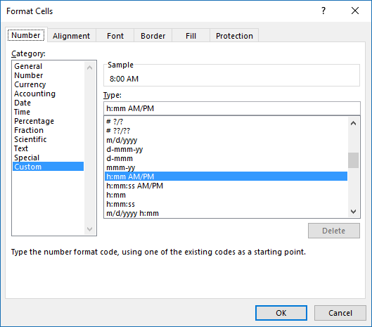
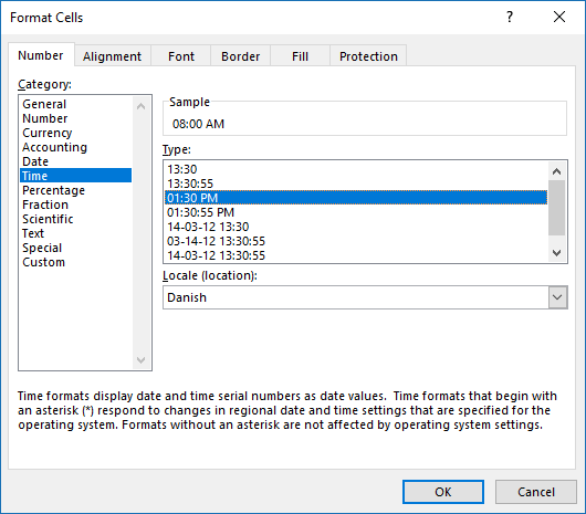
Row 1 has the following cell formatting applied:
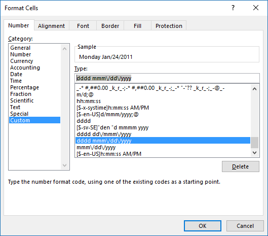
Simply select cell C1 and press CTRL+ 1 to open the "Format Cells" dialog box, shown in the above picture. dddd returns the weekday, mmm returns month name abbreviated to three letters. dd returns the day of the date and yyyy returns the year.
Formula in cell A2:
This is a cell reference to sheet Settings and cell B4.
Formula in cell A3:
Copy cell A3 and paste to cells below as far as needed.
Explaining formula in cell A3
Step 1 - Add time value to interval value
A2+Settings!$B$6
becomes
0.333333333+0.00694444444444444
and returns 0.340277777777778
Step 2 - Check if value is larger than end time
The greater than sign is a logical operator that evaluates if the value is greater than end time value, we only want time values inside the range given in sheet settings cell B3 and B4.
(A2+Settings!$B$6)>Settings!$B$5
becomes
0.340277777777778>0.708333333333333
and returns FALSE.
Step 3 - Return nothing if TRUE and date + time value if FALSE
The IF function has three arguments, the first one must be a logical expression. If the expression evaluates to TRUE then one thing happens (argument 2) and if FALSE another thing happens (argument 3).
IF((A2+Settings!$B$6)>Settings!$B$5,"",A2+Settings!$B$6)
becomes
IF(FALSE,"",A2+Settings!$B$6)
becomes
IF(FALSE,"",0.340277777777778)
and returns 0.340277777777778.
Step 4 - If above cell is empty return nothing
IF(A2="", "", IF((A2+Settings!$B$6)>Settings!$B$5, "", A2+Settings!$B$6))
and returns 0.340277777777778 formatted to 8:00 AM.
The image below shows the cell formatting applied to column A.
7. Schedule recurring expenses in a calendar
Below is an excel table containing recurring expenses and corresponding amounts, dates and recurring intervals. An excel table allows you to easily add/delete records without changing the formulas, in other words cell refs to the table are dynamic.
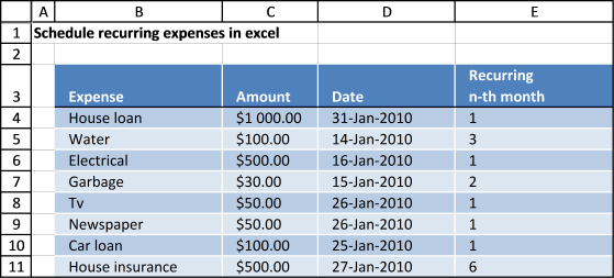
I am going to use this data set and create a calendar with each expense at the correct date (and recurring dates).
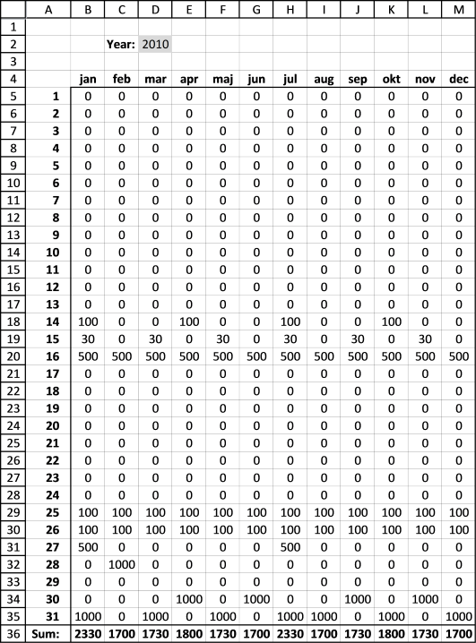
The data above is also dynamic, if you change the year in cell D2 formulas in cell range B5:M35 are recalculated.
Array formula in B5:
How to create an array formula
- Type the formula in the formula bar
- Press and hold CTRL + SHIFT
- Press Enter once
If you made it right the formula is now surrounded by curly brackets, like this: {=array_formula} in the formula bar.
Copy formula
Copy cell B5 and paste it down to cell B35.
Copy cell range B5:B35 and paste it to the right all the way to M5:M35.
Formula in B4:
Copy cell B4 and paste it right to cell M4.
Formula in B36:
Copy cell B36 and paste it to the right to cell M36.
Explaining array formula in cell B5
Step 1 - Calculate date in cell B5
DATE($D$2,MONTH(B$4),$A5)
becomes
DATE(2010,1,1)
and returns 2010-1-1 (1/1/2010)
Step 2 - Build an array of recurring dates
EDATE(TRANSPOSE(Table1[Date]), (ROW($1:$1000)-1)*TRANSPOSE(Table1[Recurring
n-th month]))
I can't show all dates here, there are two many. 1000 recurring dates for each date. I have to simplify, I am now using three recurring dates moving forward.
{40209, 40192, ... , 40570}
Step 3 - Check if current date is equal to any of the recurring dates and return the corresponding amount
IF(DATE($D$2, MONTH(B$4), $A5)=EDATE(TRANSPOSE(Table1[Date]), (ROW($1:$1000)-1)*TRANSPOSE(Table1[Recurring
n-th month])), TRANSPOSE(Table1[Amount]), "")
returns {"","",... ,""}
Step 4 - Sum values
SUM(IF(DATE($D$2, MONTH(B$4), $A5)=EDATE(TRANSPOSE(Table1[Date]), (ROW($1:$1000)-1)*TRANSPOSE(Table1[Recurring
n-th month])), TRANSPOSE(Table1[Amount]), ""))
becomes
SUM({"",...,""})
and returns 0 (zero) in cell B5.
Get Excel *.xlsx file
Schedule-recurring-expenses-in-excel-2
8. Count groups in calendar

Question:
Sam asks:
Is there a formula that can count blocks
For eg in your picture (see picture above) if the green blocks had the letter G and the Red blocks had the letter R and I had to return 4 as the answer -3G + 1R
Is this possible through a formula?
Answer:
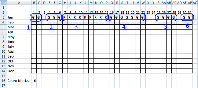
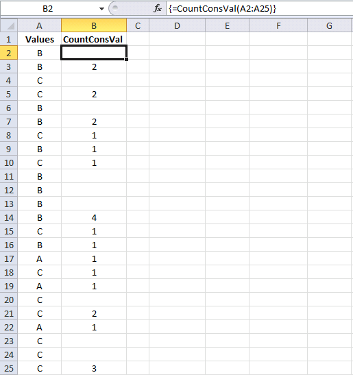
The image above shows the groups in row 3, the formula in cell B16 counts the number of groups.
Formula in B16:
Explaining formula in cell B16
Step 1 - Check if next cell is not equal to current cell
--($B$3:$AE$3<>$C$3:$AF$3)
returns {0, 1, ..., 0}
Step 2 - Check if cells are empty
--($C$3:$AF$3<>"")
returns {1, 0, ... , 1}
Step 3 - Check if first cell is not empty
=SUMPRODUCT(--($B$3:$AE$3<>$C$3:$AF$3), --($C$3:$AF$3<>""))+($B$3<>"")
($B$3<>"")
returns TRUE
Step 4 - All together
=SUMPRODUCT(--($B$3:$AE$3<>$C$3:$AF$3), --($C$3:$AF$3<>""))+($B$3<>"")
becomes =5+TRUE
and returns 6.
9. Free School Schedule Template
This template makes it easy for you to create a weekly school schedule, simply enter the time ranges and the formula takes care of the rest. See the animated image above.
The time ranges are entered in an Excel defined Table that expands automatically when new values are added, no need for dynamic named ranges.
The template has hours divided into 10-minute intervals, follow the instructions below and you will with ease create another interval if you prefer to use that.
If you don't like the look of the ranges I am using you can easily change the conditional formatting color that highlights the ranges in the schedule.
There is a workbook for you to get at the very end of this article.
How I created this dynamic template
The schedule contains formulas, conditional formatting, and an Excel defined Table, it updates instantly when you add/delete new records.
Weekdays
- Select cell G1
- Type Monday
- Select cell H1
- Type Tuesday
Repeat above steps for remaining cells and weekdays in cell range H1:M1.
10-minute intervals
- Select cell F2
- Type 8:00
- Select cell F3
- Type 8:10
- Select cell range F2:F3

If you want to use a 12-hour clock AM/PM then simply select all time values in column F and press CTRL + 1 to open a dialog box that allows you to change cell formatting.
Press with left mouse button on "Time" and then pick a format that you prefer.
Create headers
- Select cell A1
- Type Weekday
- Select cell B1
- Type Subject
- Select cell C1
- Type Start
- Select cell D1
- Type End
Create Excel defined Table
- Select cell A1.
- Press CTRL + T to create an Excel defined Table.
My table looks like this:
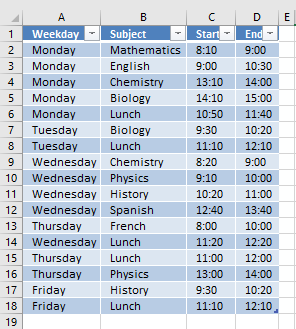
It contains some random data.
Enter array formulas
- Select cell G2
- Press with left mouse button on in the formula bar

- Type:
=IFERROR(IF(SUMPRODUCT((Table1[Start]=$F2)*(G$1=Table1[Weekday]))=0, "", INDEX(Table1[Subject], SUMPRODUCT((Table1[Weekday]=G$1)*(Table1[Start]=$F2)*(MATCH(ROW(Table1[Weekday]), ROW(Table1[Weekday])))))), "")
- Press and hold Ctrl + Shift
- Press Enter
Copy array formula
- Select cell G2
- Copy cell (Ctrl +c)
- Select cell range H2:M2
- Paste (Ctrl + v)
- Select cell range G2:M2
- Copy (Ctrl + c)
- Select cell range C3:M50
- Paste (Ctrl + v)
Create conditional formatting
- Select cell range G2:M50
- Go to tab "Home"
- Press with left mouse button on "Conditional Formatting" button
- Press with left mouse button on "New Rule..."
- Press with left mouse button on "Use a formula to determine which cells to format"
- Type =SUMPRODUCT((G$1=Weekday)*($F2=>Start))
in "Format values where this formula is TRUE" field.

- Press with left mouse button on "Format..." button
- Press with left mouse button on Border tab
- Press with left mouse button on to create three borders

- Press with left mouse button on OK
- Press with left mouse button on OK
Repeat above steps with remaining conditional formatting rules:

The border and fill formatting are also shown in the picture above.
1 : =SUMPRODUCT((G$1=Weekday)*($F2>=Start)*($F2<End))
2: =SUMPRODUCT((G$1=Weekday)*($F2=End))
3: =SUMPRODUCT((G$1=Weekday)*($F2=Start))
4: =SUMPRODUCT((G$1=Weekday)*($F2>=Start)*($F2<End))
Calendar category
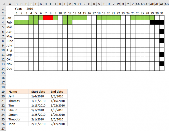
Table of Contents Plot date ranges in a calendar Plot date ranges in a calendar part 2 1. Plot date […]
This article describes how to build a calendar showing all days in a chosen month with corresponding scheduled events. What's […]
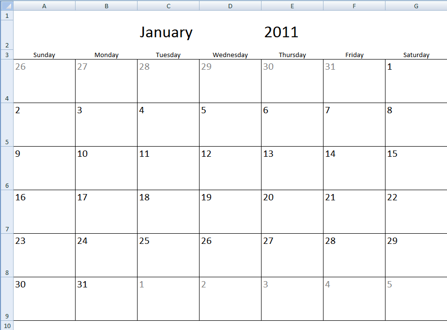
Table of Contents Monthly calendar template Monthly calendar template 2 1. Monthly calendar template The image above shows a calendar […]
If then else statement category
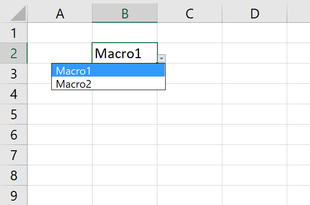
This article demonstrates how to run a VBA macro using a Drop Down list. The Drop Down list contains two […]
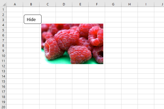
This article explains how to hide a specific image in Excel using a shape as a button. If the user […]
This post Find the longest/smallest consecutive sequence of a value has a few really big array formulas. Today I would like to […]
Macro category
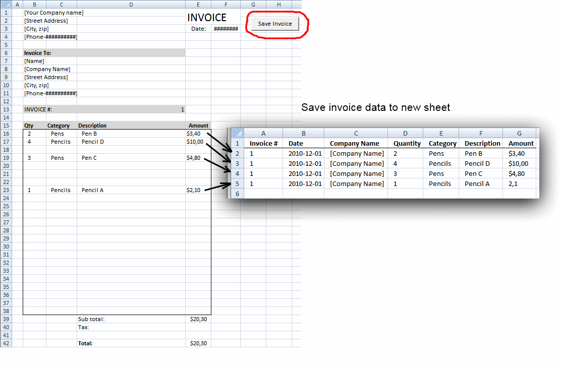
Table of contents Save invoice data - VBA Invoice template with dependent drop down lists Select and view invoice - […]
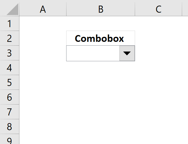
This blog post demonstrates how to create, populate and change comboboxes (form control) programmatically. Form controls are not as flexible […]
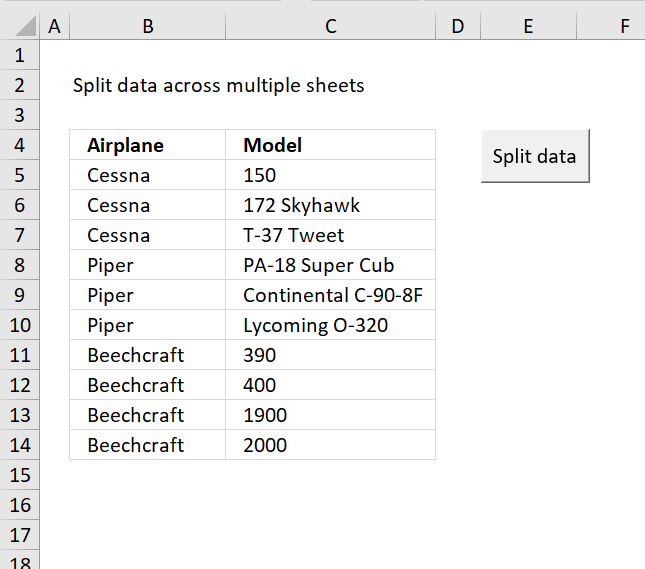
Table of Contents Split data across multiple sheets - VBA Add values to worksheets based on a condition - VBA […]
Excel categories
61 Responses to “Excel calendar”
Leave a Reply
How to comment
How to add a formula to your comment
<code>Insert your formula here.</code>
Convert less than and larger than signs
Use html character entities instead of less than and larger than signs.
< becomes < and > becomes >
How to add VBA code to your comment
[vb 1="vbnet" language=","]
Put your VBA code here.
[/vb]
How to add a picture to your comment:
Upload picture to postimage.org or imgur
Paste image link to your comment.
Oscar..Thanks for this brilliant formula.
One more question for the Calendar that you have set up above can we have a excel formula which will give us a below table
StarWk EndWk Name
1 2 G
4 6 G
7 15 R ... and so on
Sam,
Read this post: https://www.get-digital-help.com/2010/08/29/extract-dates-from-a-cell-block-schedule-in-excel/
hello,
I need your support regarding your above material - Schedule recurring expenses in a calendar.
I tried to use your formulas in LibreOffice 3.4.4(linux) and into any others OpenOffice versions but it doesn't work. It give me next errors - error 508 or #value! .
What do I have to do to convert your excel formulas into libreoffice format,please?!
Thank you in advance for your answers and helping!
In the "Calculating dates (formula)" section, Step #2... you misspelled "January" as "Janauary" in the latter part of the formula.
Thanks!
[...] number formats, and much more. Home > Excel > Automate > Use a calendar to filter a table← Previous post - Use a calendar to filter a tableFiled in Automate, Drop down lists, Excel, Search/Lookup on Sep.10, [...]
[...] How to create an Excel calendar with VBA [Get Digital Help] [...]
when i add an entry to Friday 12:30, it does not work?
TCKY,
I opened the attached excel file and added an entry to Friday 12:30 - 14:00 and it works here.
Your excel version?
hi,i am new to this blog.
but i hope i can get some help regarding a pop up calendar.
i found a pop up calendar for excel 2007,but when i try to use it in Excel 2010, the calendar does not appear. and i think it is related with the format behind.can you help me?thank you for any help and sorry for my poor English.
auni,
Do you have a link to the pop up calendar?
https://www.fontstuff.com/vba/vbatut07.htm
[...] Free School Schedule Template [...]
Hi, I would like to use this example with my data set however I'd like to visually show the amount of events per date to understand when are we the busiest, slowest, etc. and be able to forecast using this data. Ideally I would like some sort of data bar or color change indicating the level for each date (Jan 1 has 10 items while Jan 2 has 3 and I can visually see that in each cell instead of seeing numbers or a solid color for each cell (here yellow and blue).
Also, would it be possible to have Excel know the days of the month as in first 7 days of the month, last day of the month, every Monday of the month. I'd eventually like to get formulas set up to tell me on average how busy we are during these periods.
David,
Here is a basic example. It looks like a heat map.
Highlight dates VBA
Private Sub Worksheet_Change(ByVal Target As Range)
Set Rng = Range("B5:H10")
If Target.Address = "$C$2" Or Target.Address = "$E$2" Then
    'Remove previous formatting
    With Rng.Interior
        .Pattern = xlNone
        .TintAndShade = 0
        .PatternTintAndShade = 0
    End With
    For Each Cell In Rng
        For Each Value In Worksheets("Data").Range("Data1")
            If Int(Value) = Cell Then a = a + 1
        Next Value
        'Set color
        If a > 0 Then
            With Cell.Interior
                .Pattern = xlSolid
                .PatternColorIndex = xlAutomatic
                .ThemeColor = xlThemeColorAccent4
                .TintAndShade = 1 - (a / 4)
                .PatternTintAndShade = 0
            End With
        'Reset counter a
        a = 0
        End If
    Next Cell
End If
Get the Excel *.xlsm file
Calendar-David.xlsm
Contact me if you want more features.
[...] David asks: [...]
Hi there, I have opened the above calendar - and want to add another filter so I can categorize the events/meetings in the calendar, e.g. Reg for regulatory, Ben for benefits - and so when you press with left mouse button on these it will filter for that type - is this possible to do? Appreciate your help with this.
Thanks
Rosie,
Yes, it is possible. Upload a file and I´ll see what I can do.
Have you already published the code? I am very interested as i do not only want to use this, i also want to understand the reason behind it.
This looks great. I would like to use your calendar for a spreadsheet I am currently using. How could I just change where the event section refers to so it will automatically fill in the dates and times I need.
To give you context, I have a spreadsheet with many columns containing information. In these columns I have multiple dates/times for some rows. I want to create a calendar that references my spreadsheet with its events. I would like to keep all the information so that I can look at it still in the detailed view of each day (with all the information from the original row and also be able to reference the spreadsheet for multiple times for the same row but on different days).
How would I change the where the events are referenced to?
How could I add another option for dates so that I can add an extra column of values (I have the original dates column in the data sheet linked to another workbook?
[…] I got this codes from: https://www.get-digital-help.com/2012/09/05/excel-calendar-vba/ […]
Hi,
This is great and incredibly helpful!
Is there a way to modify this to schedule not just monthly, but weekly/bi-weekly/daily expenses as well? (specifically bi-weekly)
I have been looking at this as well as the post on creating a weekly schedule, but can't seem to figure it out.
Many thanks!
Dear Sir
Please I would like to know how to highlight 2nd and fourth Saturday and all sunday as weekend. Can you please suggest vba code or formula.
advance thanks.
Yours faithfully
buvanamali
[…] How to create an Excel calendar with VBA [Get Digital Help] […]
Hi,
Thank you so much for the helpful template. This is awesome! However, when I choose January, it gives me all N/A values, can you please let me know what's going on? Thanks
There seems to be an error in the Dec 31 calculation. Why is it showing $2330 when the recurring for the 31st should only be $1000? Can't seem to find where it is getting the extra amount from.
Deb,
You are right and I don't know why. I made a new smaller array formula, this one seems to work as intended.
Hi,
There seems to be a problem with values entered for the 1st of the month repeating for the last day of the month.
thanks,
Billy
I didn't understand why COLUMN($A$1:$BH$1)
Why reference to $BH$1?
Only formula COLUMN($A$1:$BH$1) gives result 1.
Nenad Deusic
I made a much smaller array formula and added a complete explanation, see article again.
Thank you for telling me.
Can you help ne with this one
=SUM(IF(DATE($d$2,MONTH(b$4), $a5)=ENDATE(TRANSPOSE Table3"DATE"),(row($45:$1000)-1)*TRANSPOSE(Table,3"recurring n-th month")),TRANSPOSE(Table3"amount")''''))
I have tried changes the prentices and quotation marks around.
Charles,
I am not sure what you are trying to do, I can't see your workbook.
If you are not familiar with excel tables read this post:
Excel Tables
I love this template. I am trying to find a way to be able to show student schedules, and I think I could use this but I would have to alter it and I'm not completely sure what I am doing. I have students that come to me for a 3 week rotation. I want a monthly calendar that will highlight the time each student is with me and then also allows me to input schedules for each day. Example student one is with me for 7/3 to 7/23, then on 7/3 they have orientation, on 7/5 they have conference and department meeting. Etc.
Emily
Have you seen this calendar?
https://www.get-digital-help.com/2016/11/10/calendar-monthly-view/
I think it will suit your requirements better.
Hi, your calendar is great for me. I want to add a new column D in the Data sheet and show the details in the calendar sheet (I added a new column right after the "Text:", how can I revise the array formula to show it properly?
Hi Oscar,
Do you have either a 2D or 3D working example of this model?
Your model is quite interesting, but I need to create a roster for (say) Patient treatments.
So my user wants to see the patient (could be a Title so that now makes it a 2D model requirement); their treatments (could be several per patient throughout a day, evening or night shift) and which staff members will perform these treatments - so constraints and rostering issues. Plus my user wants to be able to edit/modify on the go ....
How would you approach this, please?
Thank you
Murray
PS we worked on the Yahoo historic stock data issue together.
Hey Oscar,
Thanks so much for your post on the weekly schedule.
I am currently planning my school schedule and I'm having a hard time managing time conflicts/overlaps.
For example,
I have Course 1 @ 8-9 am on Monday
and Course 2 @ 8-9 am on Monday as well.
What I think might work is:
1) When a duplication occurs on the left chart (day/subject/start/end), highlight both duplication time schedules
2) If time is in 10 min intervals and a course is about 1 hr, three's enough space to both course names in the conflicting time slot in the weekly calendar
3)Another idea for 2 is that a text dialogue can be added to the sheet permanently so that if you press with left mouse button on a conflicting time slot on the weekly schedule, the names of the courses that are in conflict can be depicted there.
Anyways thanks for your time. If you have any advice on the coding or how I should go about in this project or if my ideas would even work, I would greatly appreciate your feedback.
Joseph
So I just reviewed the main formula and I realized that to see conflicts, the course start and end has to be the same.
Another issue that occurs is:
Course 1 is lets say 9:00-11:50
Course 2 is at 9:30-12:50
^That type of overlap cant be detected.
Also, the highlight formula doesn't really help play a role in this overlap situation...
Looks like some form of excel VBS might be needed.
I appreciate the time and effort for for the help. Meanwhile, Imma try to find a solution. If my solution works, I'll post it here :D
Joseph
Oscar,
Why do you create an array of 1000 recurring dates for each date? Since your calendar is only a year long, even if there was a bill each day of the year, that would only require 365?
Hi Oscar,
Great article!
I believe this knowledge is helpful especially in Finance (for recurring payment) and Maintenance (recurring preventive maintenance) industry.
I just need to ask one thing. Based on my understanding from your method, I tried to manipulate the template a bit so that the expense(or in my case, tasks) is in the left side, with the schedule at the right side (instead of days at the y axis).
I'm trying to generate forecast of recurring maintenance activity on monthly basis instead of daily basis. However, I failed where the range of the first set of array data does not match range of second set of array data in sequence. For example, using date formula, with Month in x axis, data set is {Jan 2017, Feb 2017, ...Dec 2017}. However, using edate formula (with transpose) the data set starts with whatever date the first occurrence will be, such as {March 2017, ...}
Is there any workaround for this formula so that data set with edate formula will return TRUE or any number as long as it is contained within second data set, regardless of its sequence?
Hi Oscar
Congratulations, for your job.
I would like to know, How can I do to add a field in USERFORM?
Warmest Regards
Wagner,
Try this:
https://www.excel-easy.com/vba/userform.html
Thank You!
I Want to Know how to set end date for individual expenses.
I have changed the time interval from 10 min to 15 min. Now the formatting for the following time are not working. i.e. top/bottom border and subject
15:30
16:15
17:00
17:45
18:30
19:15
19:30
20:00
example:
Monday Martial-Arts 17:00 18:00
I am missing the subject and the top border, if I change it to
Monday Martial-Arts 17:15 17:45
The bottom border is missing
So error times are the same for Start and End
Hi, I would need a help on case where event lasts for more than one day. I've managed to fix conditional formating so that color is shown well in callendar however I'm stucked on event formulas. I'd like to show first events which are from previous day and then current day ones. Could you advice how to build these table formulas correctly?
I have been searching for a way to incorporate a monthly calendar that is continuous for recurring bills which gets data from an excel spreadsheet of monthly bills. So I already have a spreadsheet with my monthly bills. I just want to add a calendar that populates with the spreadsheet information, to put it another way. Is there anything available for Excel that does this? Thank you to anyone who might be able to help!
Hi,
I am still learning excel, and hopefully you will still get a notification for this since it is about 3 years old now; but I am having the values from the 1st show up on the 31st again. How do I change that? Thank you
Hannah,
you are right. Thanks for telling me.
I have changed the formula in the article and uploaded a new file.
I found your free-school-schedule-template and find it useful but not quite what I need. I am not a newbie, nor as experienced in formulas as you are, and would love to find a solution to make my life easier.
SITUATION:
Event Staff Scheduling. When we attend events we need to schedule staff to cover the booth while others may be in meetings or attending events.
BOB =
Monday from 1-4pm and 6-8pm
KEVIN =
Tuesday from 9-12, 1-2, 3-6
Wednesday from 9-12, 2-4
SARA =
Monday from 9-1, 3-6
Tuesday from 1-3, 4-5
Wednesday from 10-1, 3-5
I tried reconfiguring your example so that the TIME BLOCKS run horizontally (top)
Names would be in rows (left side)(in reality have 25 people)
I think a Sheet for each DAY would work well
I think it would be great to have a data entry (the table you have for classes) on a separate sheet... easier to import/input the data.
Why do the first 3 conditional formatting rules apply to a different selection of cells rather than the whole table? My table is larger so the cell range needs to adjust but the top 3 appear to be applying formatting to an EMPTY section just to the right of the live table data.
Just wondering how it is used to know if I need to replicate that when I have more rows and columns. Thanks
Hi
Thank you so much for this. This has been what I have been wanting for ages. I've messaged twice over the last four days as I worked crazily on developing a dynamic timetable that imports and manipulates data from our Master Schedule and adapts it to the format needed by this timetable.
My university files are all within the Google Suite, so once I mastered the Excel version, using yours as a foundation, I went over to Google. Two days later, I succeeded in importing data dynamically and updating the timetable for each teacher in real-time.
I thought I'd share the link to the basic equivelent of a static timetable that I created in Google Sheets. It's not perfect (I have to learn about the conditional formatting of borders in Google Drive), but it might help someone else who finds this page like I did.
It also has a conflict checker built in to make sure that no two classes overlap.
Here is the link to the sheet https://docs.google.com/spreadsheets/d/16xmtGbBIrD3Irm66zIs-qJbn0dKXriiyCZV9RSGfYBI/edit?usp=sharing
Thank you again. I wouldn't have been able to achieve any of this without this webpage.
Hi Oscar,
Love the spreadsheet! Is there a way to generate the calendar for 2020 and beyond?
Go to 'Calendar' tab and select cell 'D2'
Go to the data tab at the top and hit data validation, and change 'allow' from 'list' to 'any value'.
This is epic, only I can't figure out how to make weekly or bi-weekly payments work on this one properly. They multiply to the right monthly sum, but rather spread out over 4 payments they are together as one.
Hi,
I’ve added a lot of lines of expenses to the first tab and at first the amounts were showing x1000 on the calendar for example 1000 will show as 1000000 so I adjusted the formula to divide by 1000 but now it’s showing random amounts on the calendar.
One thing to note is that I’m using vlookups to upload the expanses to the table. And I’ve also adjusted the data validation on both sheets.
Any idea for what I should different?
Thanks in advance
Thanks for share, Works great!!
Hi Oscar,
Is there a way to summarise the total monthly amount into one cell without having all of the days in the month listed as seperate rows? E.g i would like to only have 1 row which sums the total amount for all the days in the month for each month.
Thank you in advance
Thank for sharing! I was looking something like that days now!
is it possible when highlight (choose a date) it will open a new sheet? in order to enter cashier data?
And highlight red that date if all the info from the above table are completed?
The table is look like that
https://i.postimg.cc/vBxZqxcp/2021-06-22-231754.png
Also if it is possible new tab will named as the date.
Hope you understand what I am saying. (Apologies, I am Greek so English are not my native language)
Thank you!
Hi Oscar,
I've been looking for this spreadsheet for a long time. It's fantastic, thanks so much.
How do I create payments that are weekly and bi-weekly too? I'd love to be able to put all my expenses into this.
Thanks again
Hi Oscar,
I am no bright light with pivot tables but I have managed to create an excel calendar (vba) and it works great!!! Thank you so much!!!!
I have just one question as so far I have entered ones off events in it but I would like to also add recurring events (every monday there is a meeting). Short question: is that possible?