Automate net asset value (NAV) calculation on your stock portfolio
Table of Contents
1. Automate net asset value (NAV) calculation on your stock portfolio
In this post I am creating a spreadsheet that will calculate stock portfolio performance. To do this I am calculating net asset value (NAV).
Net asset value is the value of each stock and the account balance summed, calculated each day as the stock prices fluctuate.
When a deposition or withdrawal is made you add or subtract NAV units to your stock portfolio. More about deposits, withdrawals and NAV units in an upcoming post.
All other transactions affects your stock portfolio performance and is added or subtracted from your account balance.
- Stock prices
- Dividends
- Commissions
- Interest payed or earned
In this excel tutorial I will only buy or sell stocks and calculate each stock's market value (column J) each day. Dates are in column A.
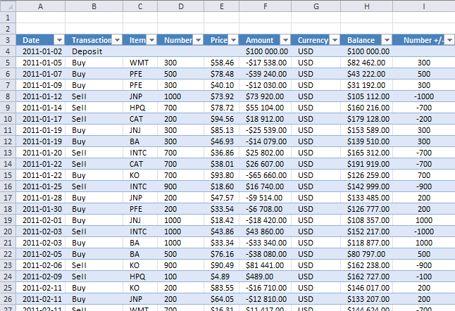
Transactions sheet
Here is the "Transactions" sheet. It contains some random stock data. Here I calculate stock portfolio market value each day.

Formula in H7:
Formula in I7:
NAV calculation sheet
In this sheet I calculate stock portfolio market value for each day. Excel queries yahoo and copies close price for each stock into E7 and down. Market value is calculated in F7 and down and the total is calculated in C4. The total is then copied into sheet "Transactions".

Formula in F3:
Formula in C3:
Formula in C4:
Formula in B7:
Copy cell and paste down as far as needed.
Formula in C7:
Copy cell and paste down as far as needed.
Formula in D7:
Copy cell and paste down as far as needed.
Formula in F7:
Copy cell and paste down as far as needed.
Web Query sheet
I created a web query in cell A5 on sheet "Web query".
https://table.finance.yahoo.com/table.csv?a=["m","m"]&b=["d","d"]&c=["y","y"]&d=["m","m"]&e=["d","d"]&f=["y","y"]&s=["ticker", "ticker"]&y=0&g=d&ignore=.csv
Parameters
y = cell P2
m = cell P3
d = cell P4
ticker = cell P5
Formula in P1:
Formula in P2:
Formula in P3:
Formula in P4:
VBA code:
Sub Calc_nav()

Application.ScreenUpdating = False

Application.DisplayAlerts = False

Dim rng As Range

Dim price As Range

Dim dest As Range

Dim mnt As Range

Dim i As Integer

Dim qryTblStocks  As QueryTable

'Iterate rows

i = Worksheets("Nav calc").Range("F2")

Set mnt = Worksheets("Transactions").Range("J7")

Do While i <= Worksheets("Nav calc").Range("F3")

 Worksheets("NAV calc").Range("C2").Value = i

 'Iterate stock symbols

 Set rng = Worksheets("NAV calc").Range("C7")

 Set price = Worksheets("NAV calc").Range("E7")

 Set dest = Worksheets("Web query").Range("P5")

 Do While rng <> ""

 dest.Value = rng.Value

 'Refresh web query

 Set qryTblStocks = ThisWorkbook.Worksheets("Web query").QueryTables(1)

 With qryTblStocks
 .Refresh BackgroundQuery:=False
 End With

 'Text to columns

 Sheets("Web query").Select
 Range("A5:A6").Select

 Selection.Texttocolumns Destination:=Range("B5"), DataType:=xlDelimited, _
 TextQualifier:=xlDoubleQuote, ConsecutiveDelimiter:=False, Tab:=False, _
 Semicolon:=False, Comma:=True, Space:=False, Other:=False, FieldInfo _
 :=Array(Array(1, 1), Array(2, 1), Array(3, 1), Array(4, 1), Array(5, 1), _
 Array(6, 1), Array(7, 1)), TrailingMinusNumbers:=True

 'Copy close value Web query F6 to NAV calc E7

 price.Value = Worksheets("Web query").Range("F6")

 Sheets("Web query").Select
 Range("A5:A6").Select
 Selection.ClearContents

 'Iterate to next cells

 Set rng = rng.Offset(1, 0)

 Set price = price.Offset(1, 0)

 Loop

mnt.Value = Worksheets("NAV calc").Range("C4")

Application.ScreenUpdating = True

Sheets("Transactions").Select

Application.ScreenUpdating = False

Set mnt = mnt.Offset(1, 0)

i = i + 1

Loop

End Sub
How to use this spreadsheet
Get excel spreadsheet: Track your stock portfolio performance.xls Remember enabling macros.
Press with left mouse button on "update" button on transactions sheet. Watch market values being calculated in column J.
Here is a picture of transactions sheet when NAV have been calculated.

Final notes
Make sure Transactions sheet is sorted by date.
Future improvements
Instead of making multiple web queries to yahoo, a better strategy would be to identify the maximum date range and then do one query for each stock in portfolio. This would also speed things up considerably.
2. Calculate your stock portfolio performance with Net Asset Value based on units
Dividends, interest, deposits and withdrawals are not calculated in this post.
The section above creates a web query to calculate Net Asset Value at any given date. Net Asset Value is cash balance in your stock account + total portfolio stock value. Dividends paid, interest earned and commissions are calculated and affects account balance. Deposits and withdrawals are not calculated in this post.
In this section we are going to calculate units of Net Asset value. Doing so we can easily calculate stock portfolio performance also when a deposit or withdrawal is made. Calculate portfolio performance by comparing your account balance day by day is wrong. Why? When you make a deposit or withdrawal, portfolio performance is distorted.
Example,
Day 1, Deposit $10 000 - Account balance: $10 000
Day 2, Buy 200 shares Caterpillar @ $40
Account balance: $9 990 ($40*200= $8000 + cash $2000 - Commission:$10 = $9 990)
Day 3, Deposit $10 000
Account balance: $9 990+$10 000= $19 990 (Caterpillar is still at $40)
The account balance has increased from Day 1: $10 000 to Day 3: $19 990 but the stock price is the same.
Portfolio performance: $19 990/$10 000 -1= +99,9%
Clearly calculating stock portfolio performance based on account balance is wrong.
Example - Net asset value based on units

Day 1, Deposit $10 000 - Account balance: $10 000.
I have chosen 100 NAV units in this example but any number will do. NAV / Units is $10 000 / 100 units = $100 per unit.
NAV/unit is the number we compare day by day to calculate portfolio performance.
Day 2, Buy 200 shares Caterpillar @ $40 (Commission $10) - Account balance: $9 990
NAV is now $9 990 and we divide with 100 NAV units equals $99,90 per unit.
Portfolio performance: 99.90/100.00 -1= -0,1%
Day 3, Deposit $10 000 - Account balance: $9 990+$10 000= $19 990 (Caterpillar is still at $40)
Account Balance = NAV. NAV is now $19 990.
NAV units increases when we do a deposit and decreases when we do a withdrawal.
NAV units increases $10 000/$99,90 = 100,1001001 units to a total of 200,1001001 units.
NAV / Units = $19 990 / 200,1001001 = $99,90
Portfolio performance: $99,90/$100,00 -1= -0,1%
(The commission is affecting stock portfolio by -0,1%.)
Excel tutorial file
In a previous related post we created a web query to calculate Net Asset Value at any given date. I have added NAV units, NAV / units and portfolio performance to the attached file.
Get excel file
Track-your-stock-portfolio-performance.xls
Excel 97-2003 *.xls
Remember to enable macros and you can´t undo a macro. Backup!

NAV formula in L7:
Copy and paste cell down as far as needed.
NAV units formula in M7:
Copy and paste cell down as far as needed.
NAV per unit formula in N7:
Copy and paste cell down as far as needed.
Portfolio performance formula:
Copy and paste cell down as far as needed. Format cells as percentage.
Recommended reading:
Compare your stock portfolio with S&P500 in excel
3. How to calculate totals of stock transactions based on dates
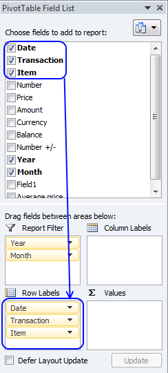
Did you know that you can use a pivot table to summarize portfolio holdings at any point in time? If you trade securities or work as an accountant this blog post is for you.
I am going to demonstrate how to sum portfolio holdings, here is a picture of the transactions table. The table contains dummy data.
I have added two columns to this table, Year and Month. This makes it possible to filter the pivot table by month and year.
Formula in cell J4:
Formula in cell K4:
Create an Excel Table
I highly recommend that you create an Excel Table, it makes life easier for you if you need to add more data to your table. This saves you time because you don't need to update the cell references, only perform a refresh the Pivot Table.
- Select all cells you want to convert to an Excel Table.
- Press CTRL + T to create an Excel Table, a dialog box is displayed.
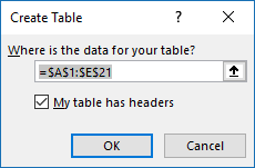
- Enable the checkbox if the Table has headers.
- Press with left mouse button on OK button.
Excel applies cell formatting to indicate that it is now an Excel Table, you can change the Table style if you want something more subtle.
Insert a Pivot Table
A Pivot Table allows you to quickly create totals based on conditions like items, dates, months, years and so on. It is one of the greatest features in Excel, in my opinion.
- Press with left mouse button on any cell in the Excel Table.
- Go to tab "Insert" on the ribbon.
- Press with left mouse button on "Pivot Table" button.

- The dialog box lets you choose the data source but the default Table is based on the cell you selected in step 1.
You also have the option to decide where you want the Pivot Table located, a new worksheet or an existing worksheet and the location on an existing worksheet. - Press with left mouse button on OK button to create the Pivot Table.

This image above shows the empty Pivot Table that we now need to configure.
How to set up the Pivot Table
Select any cell in the Pivot Table if you don't see the task pane on the right, see image above. This will open the task pane which is necessary in order to manipulate the Pivot Table.
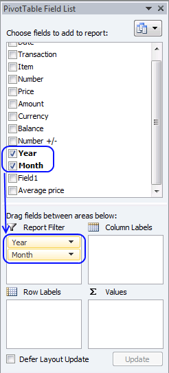
Report filter
The report filter is going to allow you to use different date ranges like years and months which is very handy in this scenario where we want to consolidate data based on stock transactions.
- Press and hold with left mouse button on "Year" field.
- Drag to Report filter area.
- Repeat steps with "Month" field.
The Pivot Table changes to this.

The Drop Down lists lets you quickly choose year and months to be included in the Pivot Table.
Row labels
The fields you drag to the row labels area will show up vertically in the Pivot Table.
- Drag Date, Transaction and Item fields to Row labels area.
- Press with right mouse button on on a date in the Pivot Table, see image below.

- Press with left mouse button on "Group..." on the menu.
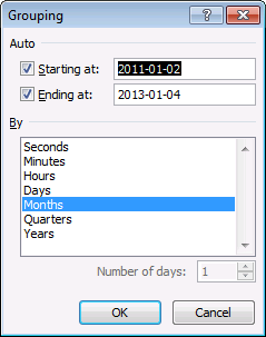
- Select "Months".
- Press with left mouse button on OK button to apply settings.
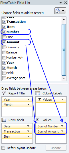
Values area
- Drag Number to the Values area.
- Press with left mouse button on Number and press with left mouse button on Value field settings.

- Select Sum, see image below.
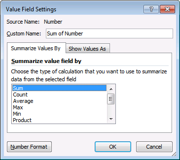
- Press with left mouse button on OK button.
- Drag Amount to Values area.
Remove Deposit from Transactions
- Press with left mouse button on Buy or Sell in the first column
- Press with left mouse button on the arrow next to Row Labels to display a menu.
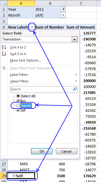
- Deselect the ceckbox next to Deposit.
- Press with left mouse button on OK button.
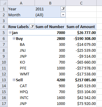
The result
Now you can examine all transactions summed month by month or if you prefer yearly.
How to sum holdings yearly
- Press with right mouse button on on a month.
- Press with left mouse button on "Ungroup..."
- Press with right mouse button on on a date.
- Press with left mouse button on Group..
- Select Years.
- Press with left mouse button on OK button.
How to refresh a Pivot Table

You need to refresh the Pivot Table if you add more values to the Excel Table later on. This is easy to forget.
4. All you need to know about calculating NAV units for your stock portfolio

This blog article explains in greater detail how to determine stock portfolio performance based on units of NAV (Net Asset Value). I made a similar blog article before (Calculate your stock portfolio performance with Net Asset Value based on units in excel) and the questions I got from that article are answered in this article.
NAV units make it easier to calculate the value of a stock portfolio if you deposit or withdraw money from your account. The value of a particular stock is changed when the markets are open, this means that NAV / unit changes when stock prices go up or down.
It is recommended to calculate NAV / unit when stock markets are closed using the closing prices of the stocks you have in the portfolio. You can then monitor the performance of your stock portfolio day by day.
Day 1 - Deposit money
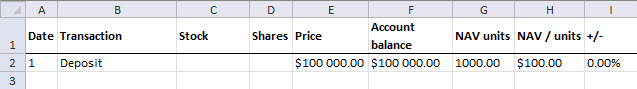
Today you deposit $100 000 to your account meaning you add money $100 000 to your broker account. A stockbroker is a firm that buys or sells shares or other securities based on what you tell them to do. They often accept orders by phone calls or a trading application through the internet.
I use 1000 NAV units in this example but you can use any number you like here. NAV is $100 000 and NAV / unit is $100 000 / 1000 = $100 per unit.
Formula in cell H2:
Day 2 - Buy a stock
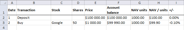
On the next day you buy 50 Google shares and they cost $1000 each. You pay $10 in commission. You now have $100 000 - 50*$1000 -$10 = $49 990 in cash in your account.
The stock is worth the stock price multiplied with the number of shares you own, in this case, 50 shares. $1000 * 50 shares = $50 000. Your NAV (account balance) is the value of the stocks plus the cash in your account, $50 000 + $49 990 = $99 990.
You have 1000 NAV units and the NAV / unit is now $99 990 / 1000 = $99.90. Portfolio performance is 1 - 99.9/100 = -0.1%.
Why did the stock portfolio decrease in value? You paid $10 in commission.
Formula in cell I2:
$H$2 is an absolute cell reference meaning it won't change when you copy the cell and paste to cells below. On the other hand, H2 is a relative cell reference and it will change when you copy and paste the cells to cells below as far as needed.
Column I shows the performance from date 1 and not based on the prior day or the prior calculation. To calculate the performance day by day use this formula in cell I3:
Both cell references are relative and will change when you copy the cell to cells below.
Day 3 - Withdrawal
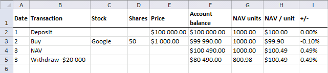
Google share price is today $1010. Your stocks are now worth 50 * $1 010 = $50 500. You have $49 990 in cash and your account balance is $50 500 + $49 990 = $100 490.
NAV / unit is $100 490 / 1000 = $100.49. Portfolio performance is 1 - 100.49/100 = 0.49% This article explains how to
You have $49 990 in cash and you have decided to withdraw $20 000 from your account. The cash is now $49 900 - $20 000 = $29 990. A deposit or withdrawal affects your NAV units. How many NAV units?
$20 000 / $100.49 is approximately 199.02 NAV units. 1000 - 199.02 is approximately 800.98 NAV units.
Despite the fact that the account balance is lower than the day before, your stock portfolio performance is still up 0.49% compared to day 1.
Day 4 - Dividend
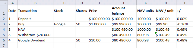
You receive a dividend $10 per share. A dividend is a cash payout from the company to the shareholders which is common if the company is profitable.
50 * $10 = 500. Your cash is now $29 990 + $500 = $30 490.
Your Google shares are now worth $1 007 per share. 50 * $1007 = $50 350. Your account balance is $30 490 + $50 350 = $80 480
Dividends affect NAV / unit. NAV / unit = $80 480 / 800.98 is approximately $100.48
The stock price went down from $1010 day 3 to $1 007 today (day 4), however, you also received a dividend that increased the NAV value.
Day 5 - How is your stock portfolio doing today?
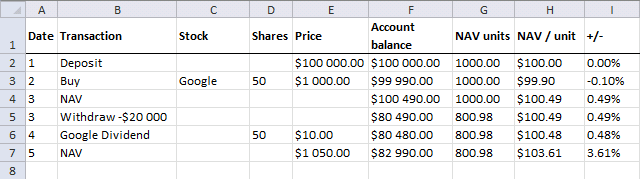
Google is now at $1050. $1050 * 50 = $52 500. Your have $30 490 in cash. $52 500 + $30 490 = $82 990.
$82 990 / 800.98 is approximately $103.61. Your portfolio is up 3.61%
Day 6 - Deposit $20 000
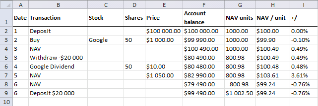
Google is now at $980. 50 shares * $980 = $49 000. Your have $30 490 in cash. $49 000 + $30 490 = $79 490. NAV / unit is $79 490 / 800.98 = $99.24. Your portfolio is down -0.76%
Deposits affect NAV units. $20 000 / 99.24 is approximately 201.23 NAV units. 800.98 + 201.23 = 1002.50 units
You now have $30 490 + $49 000 + $20 000 = $99 490. The portfolio is down -0.76%, however, your account is now worth more than day 5 because of that deposit you made.
Day 7 - Sell stock
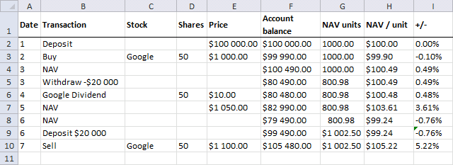
Today you sell Google stock at $1100. 50 shares * $1 100 = $55 000. You have $50 490 in cash - $10 in commission + $55 0000= $105 480.
Selling a stock affects NAV / unit. The NAV (account balance) is $105 480 and NAV units are $1002.50.
$105 480 / 1002.50 is approximately 105.22 Your portfolio is up 5.22% compared to day 1.
Day 8 - Short selling a stock
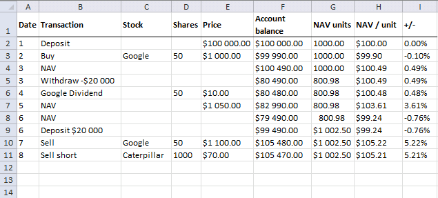
Short selling means that you borrow shares from someone and return the shares at some point in the future. This allows you to sell the stock shares and then, later on, buy them back.
This is something you can do when you believe the share price is going to go down. Today you sell 100 shares of Caterpillar at $70. $105 480 -$10 = $105 470.
NAV / unit is $105 470 / $1 002.50 = $105.22 Your portfolio is up 5.21%
Day 9 - How is your stock portfolio doing today?
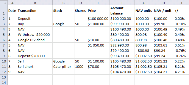
Caterpillar is at $71. $70*1000 - $71*1000 = -$1000. $105 470 - $1000 is $104 470
$104 470 / $1 0002.50 = $104.21. Portfolio is up 4.21% from date 1.
Day 10 - Buy stock
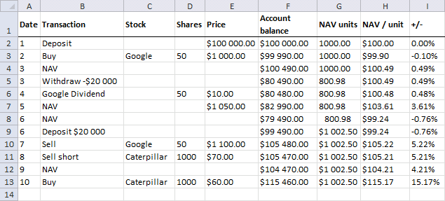
Today you buy 1000 shares of Caterpillar at $60. The share price is lower than day 9 so you made a profit.
The NAV value is $105 470 + $70*1000 -$60*1000 -$10 = $115 460. NAV units are $1 002.50. The NAV / unit is $115 460 / $1002.5 = $115.17
The stock portfolio is up 15.17% from the start.
Remember
- Deposits and withdrawals change NAV units.
- Stock value, dividends and commissions change NAV / unit.
Get Example file *.xlsx
Stock portfolio category
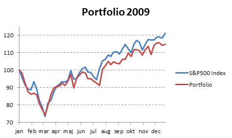
Table of Contents Compare the performance of your stock portfolio to S&P 500 Tracking a stock portfolio in Excel (auto […]
Excel categories
52 Responses to “Automate net asset value (NAV) calculation on your stock portfolio”
Leave a Reply
How to comment
How to add a formula to your comment
<code>Insert your formula here.</code>
Convert less than and larger than signs
Use html character entities instead of less than and larger than signs.
< becomes < and > becomes >
How to add VBA code to your comment
[vb 1="vbnet" language=","]
Put your VBA code here.
[/vb]
How to add a picture to your comment:
Upload picture to postimage.org or imgur
Paste image link to your comment.
How are you tracking option buys and sells, also how are you dealing with short positions?
Matt,
This excel sheet gets price quotes from yahoo and it tracks neither shorts nor options.
Can the sheet be used for non US stock?
Buzz,
Yes, if the stock has a ticker symbol in yahoo.
How do I get your excel software?
Thank you!! I have one account and in it I have a portfolio of stocks and a portfolio of bonds. Your spreadsheet makes it very eazy to track the performance of both portfolios separately even with multiple activities associated with each portfolio. Before It was very labor intensive to keep the two portfolios individually since they were in the same brokerage account. One could track many sub portfolios just by setting up your NAV spreadsheet for each one and checking to make sure the sum of the sub portfolio's NAV was equal to the brokerage account NAV.
It also will be eazy to reallocate between the two just by changing the Start values from say 80/20 to 60/40 or whatever in the spreadsheet. After resetting the start values the ending cash values will tell me how much to move between the portfolios and not destroy my previous daily accounting. Great!!!
I put you on my favorites list :D
John Prather,
I am really happy you found it useful!
Actually, I have found that with the two portfolios you just sell/withdraw one and deposit/buy the other to reallocate. Don't mess with the start values. That way your historical NAV information is unaffected so if you are graphing the data, the graphs stay intact through the reallocation. Certainly an important upgrade to my past efforts and very efficient time wise. I just down load the daily activity from Interactive Brokers and plug in the info (buys, sells, dividends, accured dividends, fees, and commissions) into the two NAV sheets and my portfolios are nicely separated so that performance of each is trackable.
To repeat Ron Temko's Question:
How and where can I get your Excel workbook??
To repeat Ron Temko's Question:
How and where can I get your Excel workbook?? It looks to be useful.
Prof. Michael Adler,
I can open the file here. If it doesn't work, try later or email me.
Track-your-stock-portfolio-performance.xls
Hi, The spreadsheet you provided in your comment above "Track-your-stock-portfolio-performance.xls" gives Runtime Error'1001' when I press with the left mouse button on update "Unable to open: table.finance.yahoo.com/..."
thanks, Uday
uday
It is well known that Yahoo made significant changes to their US website in mid May 2017. A lot of people were left high and dry most of the price look up does not work any more and there are no straight forward work arounds. If you find one please post
I am using this now on several portfolios within one brokerage account. I have learned that by carefully selecting the number of NAV units in each portfolio you can make them all have the same NAV/unit at the start. Doing this allows for easy graphing of the portfolios vs time to get relative performance. Vey nice Spread Sheet.
[...] stock portfolio performance. I am going to use Net Asset Value based on units in this post.Automate net asset value (NAV) calculation on your stock portfolio (vba)Calculate your stock portfolio performance with Net Asset Value based on units Transfer data We need [...]
[...] based on units in this post.Automate net asset value (NAV) calculation on your stock portfolio (vba)Calculate your stock portfolio performance with Net Asset Value based on units Transfer data We need monthly data from both the stock portfolio and S&P 500. First open [...]
Very helpful sheet but I have 2 issues I have been having trouble with. Hopefully you can lend some expertise, which would be greatly appreciated.
1 - My trades have either 1 or 2 exits, so trades can take 1 or 2 lines. I was able to write
Exit 1 - =IF(D9>0,(IF((C9="L"),(G9-E9),IF((C9="SS"),(E9-G9)))),(IF((C9="L"),(G10-E9),IF((C9="SS"),(E9-G10)))))
Exit 2 - =(IF((C10="L"),(G11-E10),IF((C10="SS"),(E10-G11))))
Where C=L/SS (long or short), D=Quantity, E=Entry Price, F=Exit Date, G=Exit Price.
I need to calculate the amount invested every day. There will be new positions, partial exits, full exits to be calculated, based on the entry date (Column A) and exit dates (Column F) while the amount invested in each trade will be based on entry size (Column D) minus exited size (Column H) and entry price (Column E) plus or minus the previous amount invested.
2 - Is there an easier way to write the formula calculating Exit 1 and Exit 2 so that I don't have to manually see if the trade had 1 or 2 exits and paste the correct formula, but allow it to determine if its a 1 or 2 line trade and use the correct part of the formula? Thanks.
=YEAR([@Date]) looks like SQL, could you please explain what it does, and how it does it?
Cyril,
It is a cell reference inside the table. [@Date] returns the value from the Date column and same row.
Yes, a year(a1) would be translated into a year([header]) in a table, just wondering if this could be used beyond tables... Hence if the use of @ is limited to tables within excel.
Yes, a year(a1) would be translated into a year([header]) in a table
year([header]) is a reference to the entire (table) column: [header].
just wondering if this could be used beyond tables... Hence if the use of @ is limited to tables within excel.
Yes, @ is limited to tables, as far as I know.
Hi Oscar,
You have a great excel sheet here. I have been working with it for few days to make it work with Indian stocks (I also experimented using Google API as they seemed more reliable and simple for Indian stocks).
I've been hitting roadblocks which I have been able to surpass, but I have a doubt now which I am unable to get the answer of.
This is in reference to the column NAV (K in the excel sheet shown above):
If I understand correctly, you are calculating NAV and NAV units progressively as the person had purchased/sold stocks.
So the "NAV" and "NAV Shares" is corresponding to the point of time when the transaction was made.
And the column "Total Stock Value" is corresponding to its current value.
However, I see that "NAV" formula has a reference to the "total stock value" column too while determining the NAV. That doesn't seem right to me. It means that NAV and NAV shares will be different for a transaction each time I run the "Update".
Can you please clarify?
Thanks,
Mukesh
Mukesh,
However, I see that "NAV" formula has a reference to the "total stock value" column too while determining the NAV.
Yes, Net asset value is the value of each stock and the account balance summed, calculated each day as the stock prices fluctuate.
That doesn't seem right to me. It means that NAV and NAV shares will be different for a transaction each time I run the "Update".
That is not happening here. The values are the same each time I press the "Update" button.
Thanks Oscar. Yes, NAV will be different each day for each stock. I was misinterpreting earlier.
However "NAV shares" shouldn't be different each day. Right?
For some reason the 'update' is not working in the excel sheet right now here, but this is the formula in the cell#M24
=M7-(F8="Withdrawal")*(-H8/((I8+J8-H8)/M7))+(F8="Deposit")*(H8/((I8+J8-H8)/M7))
You see this has a reference to J8, and that would mean that "NAV shares" would be different each day. Isn't it?
PS: I was actually using your other sheet in https://www.get-digital-help.com/calculate-your-stock-portfolio-performance-with-net-asset-value-based-on-units-in-excel/
Somehow posted here as the excel snapshot looked same.
Sorry, the cell I was referring to was M8
You would see that here the NAV units would not change on refresh as the rows are not for "Deposit" or "Withdrawal". However the cell M24 has Deposit, and I think that would come out different each day.
Mukesh,
However "NAV shares" shouldn't be different each day. Right?
From https://www.fool.com/foolfaq/foolfaq0056.htm:
When you deposit or withdraw cash, you treat it as though you are buying or selling the NAV units -- that is, you add or subtract the appropriate number of units.
=M7-(F8="Withdrawal")*(-H8/((I8+J8-H8)/M7))+(F8="Deposit")*(H8/((I8+J8-H8)/M7))
You see this has a reference to J8, and that would mean that "NAV shares" would be different each day. Isn't it?
It would change if it is a withdrawal or a Deposit that specific day.
Hi Oscar,
Thanks for the reply. Sorry for writing in late.
I am sorry but I am still not convinced. I feel that with this method value in the "NAV shares" column for a row corresponding to 21 june 2009 (or any other old date) would be different on 13 Mar 2013 and 14 Mar 2013, which I think is not desirable (even after reading the article that you gave reference of).
Is it possible that we connect up on chat somewhere to clarify this? Please let me know. My email id mghatiya AT gmail
Thanks,
Mukesh
Mukesh,
I am sorry but I am still not convinced. I feel that with this method value in the "NAV shares" column for a row corresponding to 21 june 2009 (or any other old date) would be different on 13 Mar 2013 and 14 Mar 2013, which I think is not desirable (even after reading the article that you gave reference of).
I don´t have those dates in my workbook or what workbook are you refering to?
Those are some dates I just cooked up.
Mukesh
Ok, I don´t know how to describe this in greater detail. Read the article again and contact the author: https://www.fool.com/foolfaq/foolfaq0056.htm
Sure. I was just trying to say that market price of today should not affect the NAV that I computed in past (for transaction that I did then).
Anyway, sorry that I have been unable to communicate it well.
I'll probably read up more.
Thanks for your time to look into it.
Sorry, I meant to write "I have NOT been able to communicate it well" :)
Hi,
In your sheet, there is only one "Deposit" in the beginning and none after that. Hence the "0" row in your "NAV Calc" sheet comes in last. However, I have deposit in between too. Because of that the "0" row is coming in between.
In your VBA code you have condition for
Now because of this the loop stops as soon as the "0 row" is hit.
To solve this, I thought I would name that row as "blank" and say loop can continue if the "blank" is hit. However, I just figured that there is no "continue" in VBA. I tried GoTo, but it is not working for me. I have no background of VBA, so unable to see what can be done. Can you guide a bit there?
Cheers,
John
John,
Upload an example file
Hi Oscar,
I like this Spreadsheet and I'm trying to use it to track with IRA account which consist of both Mutual Funds and Stocks.
I haven't been able to get it to work to update Mutual Funds off Yahoo.
Is there something special that needs to be done to allow for the combination of Mutual Funs and Stocks?
Thanks
Anil R.
Here is an example using both stocks and a mutual fund.
Track-your-stock-portfolio-performance-mutual-funds.xls
Hi Oscar,
I'm trying to figure out how you calculated the "Total stock Value" in column "J".
It seems like it is based on the end-of-day Stock Price; but I played around with the end-of-day Stock Price for "CAT" of $56.99 on 2/1/2009 and cannot come up to your number, $18,764.00
Can you help me understand your calculations in Column "J"?
Thanks.
Anil R.
It seems like it is based on the end-of-day Stock Price; but I played around with the end-of-day Stock Price for "CAT" of $56.99 on 2/1/2009 and cannot come up to your number, $18,764.00
The closing price for "CAT" 1/2/2009 was 46.91.
I think you got the date wrong.
Sorry about that Oscar. You are right. I got the date wrong. "My bad"
Cheers!
john,
i am in the process of trying to set this up. I am confused a bit about the second page and what needs to be input here ? or does it simply pull from the main page where everything is entered? Also, is it possible to pull data from Intereactive brokers instead of yahoo?
any extra help would be appreciated
thanks,
wyatt
john,
ok figured out my last questions. Running into two issues. Will it affect the data if i short stocks and have shorts in the portfolio?
When i press the "update button" the spreadsheet locks up on me, and i have to force it to close, for it never recovers", any thoughts?
Since you are far more ahead of my excel skills, can you write a simple formula that will give me percentage of returns automatically whether it is a buy or sell? i am assuming that somewhere in the equation, there has to be IF=BUY, then, or IF = Sell then....just to get the math right when getting percentage returns. I have racked my brain and cannot figure it out
thanks for any help you can provide. I see that the last commetns were quite sometime back, hope your still around
cheers,
wyatt
[…] Automate net asset value (NAV) calculation on your stock … – Introduction In this post I am creating a spreadsheet that will calculate stock portfolio performance. To do this I am calculating net asset value […]
Hi Oscar,
I was looking through the file, and I was wondering where the file was calling the data form yahoo? I looked in the macros but couldn't find a web query.
Hi Oscar,
I just opened your file and opened it in Excel 2016 and got this error as soon as I hit button Update:
Run Time error.
Unable to open:
https://table.finance.yahoo.com/table.csv..
Cannot locate the Internet Server
Then, I pressed with left mouse button on debug and it gave me this error in Yellow:
.Refresh BackgroundQuery:=False
Thanks for your Help!
Stephane
Stephane
Yahoo made significant changes to their US website in mid May 2017, you need a workaround to transfer quotes data.
Read here: https://www.xlautomation.com.au/free-spreadsheets/yahoo-historical-price-extract
Thank you Oscar. However I tried to integrate with your actual VBA without success. I am not a developer, so it is possible to send an updated Excel version with this new connection integrated?
Thanks in advance
Regards
Stephane
So when we sell some shares, we have to deduct the NAV units from the total NAV units right?
Akshay
Yes
Hi,
this was really helpful.
One question though - what happens when we sell the stock?
If we sell something in a loss, then also units are reduced and NAV increases?
Hi,
I've been using your spreadsheet for 10 years. Thank you. Its great. I update it on the 30th of every month with any withdrawal/deposit plus put in the new total value of my portfolio. I don't track individual stocks in this. I just treat my portfolio like a mutual fund and this spreadsheet has helped me to understand performance year by year. I update the contributions made and portfolio value each month with one line item.
As I've been relooking at this, I have a question about Column M that is confusing me. If I deposit or withdraw in the month, the updated # NAV units is affected by both the deposit/withdrawal amount and the new gains/losses in the portfolio. WHen I do a trial and deposit money but assume the portfolio value was unchanged (no gain or loss in the month) I get a different number of NAV units added/subtracted than if I update the portfolio value at the same time. Can you explain this please?
Thanks
Craig
Craig,
I am not sure I understand, you get a different number of NAV units because your portfolio value has changed during the month?
For example, day 3 above has this comment: (Caterpillar is still at $40)
This makes the example calculation easier, we only have to calculate the new number of NAV units for day 3.
However, if Caterpillar was at $38 at the end of the day 3 the NAV becomes 38*200 = 7600 + 1990 = 9590. NAV/units is 95.90. The deposit is $10000 and 10000/95.90 = 104.27528 additional units. The total number of NAV units is now 104.27528 + 100 = 204.27528.
For some weird reason the NAV sheets gets all the number of shares 0 from row 22? I've spent hours searching, can't find an error?