5 easy ways to extract Unique Distinct Values

First, let me explain the difference between unique values and unique distinct values, it is important you know the difference so you can find the information you are looking for on this web page.
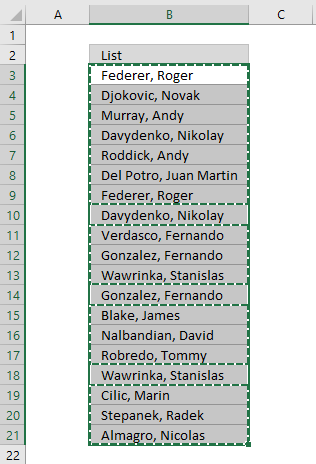
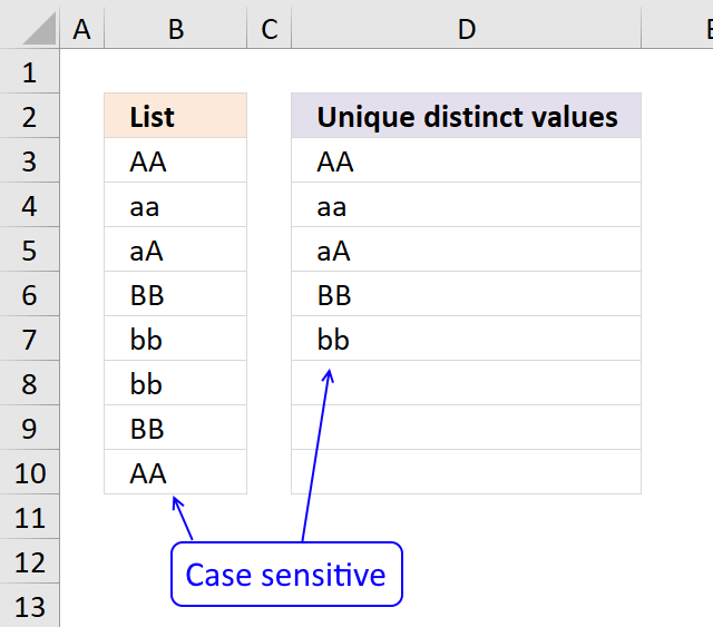
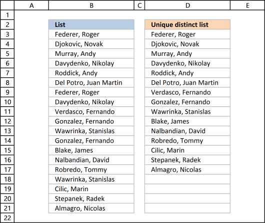
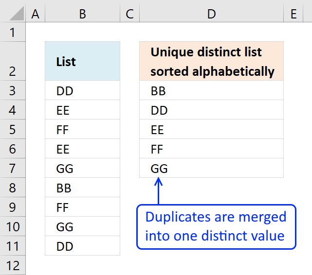
The picture above shows a list of values in column B, note value AA has a duplicate. Unique distinct values are all cell values but duplicate values are merged into one distinct value. In other words, duplicates are removed only one instance of each value is left in the list.
Column F contains unique values from column B, meaning values that exist only once in column B. Value AA is not in column F because it has a duplicate, in other words, AA is not unique in column B. To filter duplicates, read this post: Extract a list of duplicates from a column
Table of Contents
Working with unique distinct values
- How to extract unique distinct values from a column [Formula]
- Extract unique distinct values (case sensitive) [Formula]
- Filter unique distinct values [Advanced Filter]
- Highlight unique distinct values [Conditional Formatting]
- How to hide duplicate values [Conditional Formatting]
- Put unique distinct values at the top of the list [Conditional Formatting]
- Extract unique distinct sorted values from a cell range [UDF]
- Filter unique distinct values from multiple sheets [Add-In]
- How to extract unique distinct values from a column [Old array Formula]
- Create a unique distinct list using Advanced Filter in a macro - VBA
- Filter unique distinct values - case sensitive - UDF
Working with unique values
- How to filter unique values from a list [Formula]
- Highlight unique values [Conditional Formatting]
- Useful tips
- Remove errors, Excel version 2007 and later
- Remove errors, Excel version 2003 and earlier
- How to ignore blank cells
What you will learn in this article
- The difference between unique distinct values and unique values.
- How to decide which Excel feature to use.
- How to use a formula that extracts unique distinct values.
- How to copy the values returned by the formula.
- How the formula works and the functions being used.
- How to filter unique distinct values considering lowercase and uppercase letters.
- How to filter unique distinct values using the Advanced Filter.
- How to highlight unique distinct values using Conditional Formatting.
- How to build a User defined Function that filters unique distinct values sorted from A to Z.
- Where to put the VBA code.
- How to enter and use the User defined Function.
- How to filter unique values using a formula.
- How to highlight unique values using Conditional Formatting.
What is possible with formulas?
You have quite a few options to choose from if you are looking for a way to create a unique distinct list in your workbook, all demonstrated in this post or on this website. Not only an exceptionally small regular formula, if you want to use that, but also awesome built-in features in Excel that makes your work so much easier.
Formulas are very versatile, they allow you to build solutions for very specific tasks like filtering unique distinct values from two separate columns or three. If your list contains blanks then this article is for you: Extract a unique distinct list and remove blanks
Perhaps you want to do a wildcard lookup and return unique distinct values or simply return unique distinct values based on a condition.
I have also written articles that explains how to create a unique distinct list sorted alphabetically, sum or frequency.
There is also a formula for extracting unique distinct values located in a multi-column cell range, it is a somewhat more complicated array formula, however, there is a custom function as well, if you prefer that.
What is the easiest way to filter unique distinct values?

I would choose the advanced filter if you are not looking for a formula. It lets you quickly filter a unique distinct list.
If you know that you will be extracting unique distinct values from time to time, like in a dashboard or an interactive worksheet, I recommend using a formula and an Excel defined table. You won't need to repeat the same steps over and over compared to the advanced filter and that will save you time and repetitive work.
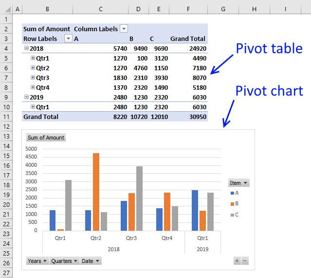
However working with a large data set may slow down the formula calculations considerably depending on your computer hardware, so perhaps the User Defined Function [UDF] is a better choice or even better a pivot table, if you have huge amounts of data to work with.
The Excel Pivot table is lightning fast even with huge data tables but it does have a little learning curve and it requires a few steps to set it up but in my opinion, it is totally worth learning how to use pivot tables. You will be surprised how easy it is to start working with Excel Pivot tables.
Conditional Formatting allows you to format cells determined by a built-in rule or a formula you construct. In this post, you will find a Conditional Formatting formula that highlights unique and unique distinct values. Did you know that you can easily sort highlighted values on top? Check out conditional formatting.
I have made an add-in that lets you extract unique, unique distinct and duplicate values and records from multiple worksheets. This allows you to easily bring together data from multiple sources in your workbook.
There is also a useful array formula in this article that extracts a case-sensitive unique distinct list, this is a special case which the built-in Excel tools can't accomplish.
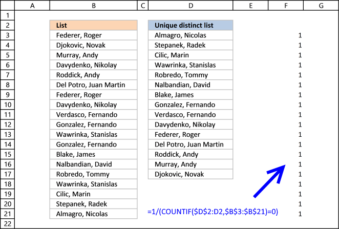
1. Create a list of unique distinct values
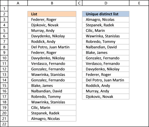
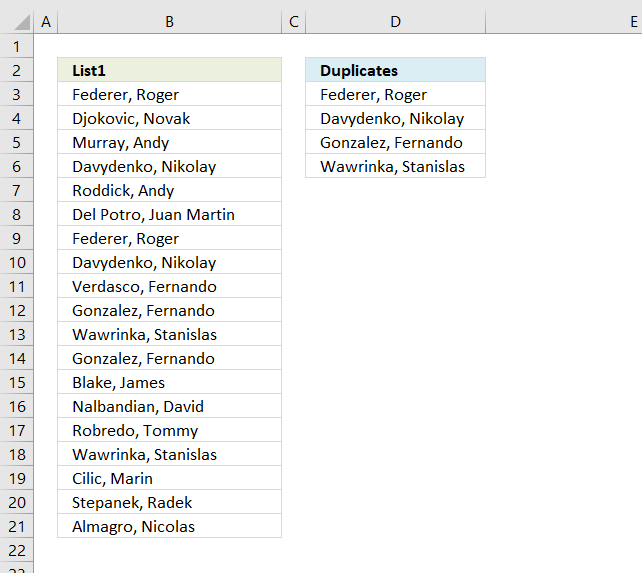
Column B contains names, some cells have duplicate values. A formula in column D extracts a unique distinct list from column B.
Update: 2017-08-15!
This formula is even smaller than the array formula and you are not required to enter this as an array formula. The following formula is for older Excel versions than Excel 365 subscribers.
Formula in cell D3:
I will explain how this formula works in the video below and in section 1.3 also below.
Update: 2020-05-28!
Microsoft Excel released new functions for Excel 365 subscribers in January 2020. One of those new functions is the UNIQUE function, it allows you to easily extract a unique distinct list using only one function.
Formula in cell D3:
This formula is entered as a regular formula, however, it is a dynamic array formula. Microsoft Excel introduced dynamic array formulas in January 2020 as well.
Dynamic array formulas expand to cells below automatically if more than one value is returned from the formula. Microsoft Excel calls this behavior spilling. You can find more example of the UNIQUE function here.
I will describe a formula for older Excel versions below.
Extract unique distinct values - Excel 365 (Link)
Extract unique distinct values sorted from A to Z - Excel 365 (Link)
Extract unique distinct values ignoring blanks - Excel 365 (Link)
Extract unique distinct values sorted from A to Z ignoring blanks - Excel 365 (Link)
1.1 Video
This video demonstrates how to use the formula:
[adthrive-in-post-video-player video-id="YnwCnhIb" upload-date="2020-05-27T07:26:00.000Z" name="Extract unique distinct values" description="How to extract a unique distinct list using a formula" player-type="default" override-embed="default"]
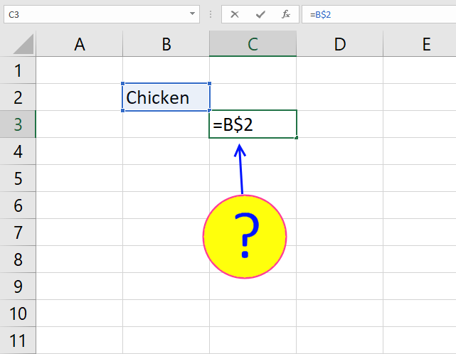
1.2 Copy unique distinct values
To copy unique distinct values to another location you must make sure you copy the values and not the formula:
- Select list
- Copy list, shortcut keys: CTRL + C or press this button:
- Press with right mouse button on on destination cell and press with left mouse button on the black arrow next to "Paste Special..."
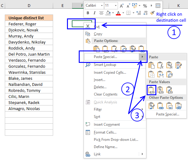
- Then press with left mouse button on "Paste Values" button.
1.3 Explaining formula in cell D3
Step 1 - Count previous values above the current cell
The COUNTIF function allows you to count values based on a condition. With the help from an expanding cell reference, the formula knows which of the values that have been extracted.
In cell D3 no values have been extracted so it compares the value in the cell above current cell, this happens to be the Header value. Make sure you don't have a value in the list that matches the header value, it won't be extracted.
COUNTIF($D$2:D2,$B$3:$B$21) is entered in column F, displayed in the picture below.
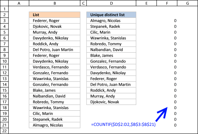
The value in cell D2 is not found in any instance in cell range B3:B21, all values in the array are 0 (zero). Note that the array has the same size as the list in column B, 19 values.
Step 2 - Compare array with 0 (zero)
To identify values that have not been shown the formula compares the array with 0 (zero) and the result are boolean values (TRUE or FALSE) for each value in the array.
COUNTIF($D$2:D2,$B$3:$B$21) = 0
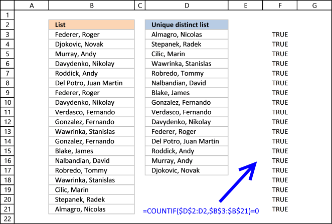
The array contains 19 boolean values, all TRUE.
Step 3 - Divide 1 with array
The boolean value TRUE is equal to 1 and FALSE is equal to 0. If a value in the array is TRUE the result will be 1 because 1/TRUE equals 1.
If a value in the array is FALSE the result will be #DIV0! because 1/FALSE is 1/0 and you can't divide a number with zero. Excel returns an error.
The good thing about the LOOKUP function is that it ignores errors, see next step.
Step 4 - LOOKUP value
The LOOKUP function is designed to work with sorted cell ranges or arrays, you get weird results if they are not sorted. Be careful using the LOOKUP function.
However, in this case, the values in the array are either 1 or #DIV0!. Surprisingly it ignores errors, the only thing it can find then is a value that is 1.
The first argument in the LOOKUP function is 2 so the function finds the last largest value that is equal to 2 or smaller.
LOOKUP(2,1/(COUNTIF($D$2:D2,$B$3:$B$21)=0),$B$3:$B$21)
becomes
LOOKUP(2,{1;1;1;1;1;1;1;1;1; 1;1;1;1;1;1;1;1;1;1},$B$3:$B$21) and matches the last value in the array. LOOKUP function then returns the corresponding value in cell range $B$3:$B$21 which is Almagro, Nicolas
1.4 Excel file
Extract a unique distinct list sorted from A to Z
Extract a unique distinct list sorted from A to Z ignore blanks
Vlookup – Return multiple unique distinct values
Unique distinct list sorted alphabetically based on a condition
Extract a unique distinct list from two columns
Extract a unique distinct list from three columns
Filter unique distinct records
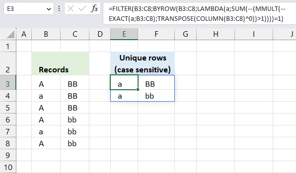
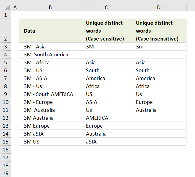
2. Extract a unique distinct list (case sensitive)
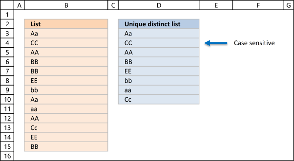
The following array formula lists unique distinct values from a list also considering upper and lower letters. For example, the value "Aa" is not equal to "AA".
Array formula in cell D3:
Excel 365 subscribers can use this regular somewhat shorter formula in cell D3 than the formula below:
The formula above contains two new formulas: LET function and the SEQUENCE function.
2.1 Video
This video demonstrates how to build a formula that extracts a case-sensitive unique distinct list:
[adthrive-in-post-video-player video-id="zqqkMntw" upload-date="2020-05-27T08:38:01.000Z" name="Extract a case sensitive unique distinct list" description="How to extract a case sensitive unique distinct list" player-type="default" override-embed="default"]
Subscribe to Get Digital Help on Youtube:
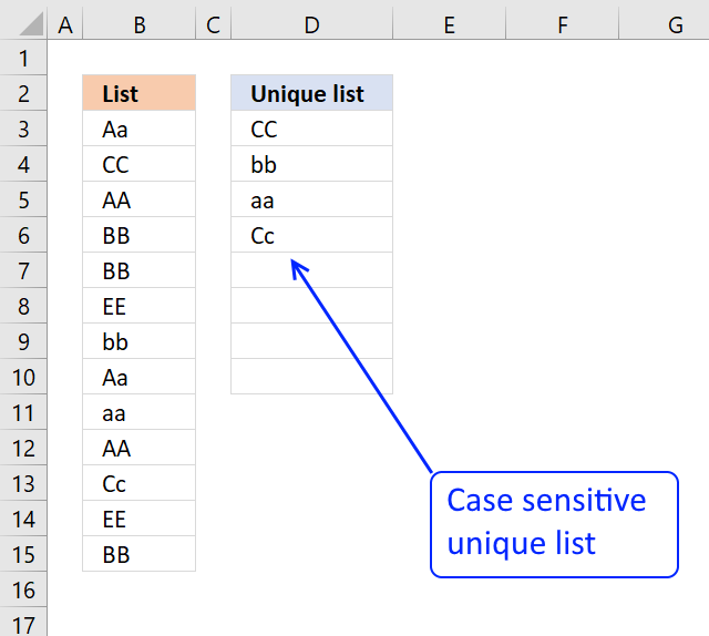
This post shows you how to extract a case sensitive unique list from a column:
Recommended articles
This article demonstrates a formula that extracts unique values from a column also considering upper and lower characters (case sensitive). […]
2.2 Explaining the array formula in cell C3
Step 1 - Transpose previous values
TRANSPOSE($D$2:D2)
returns
{"Unique distinct list (case sensitive)","Aa"}
Note that the ; (semicolon) changes to a , (comma)
Recommended reading:
Recommended articles
What is the TRANSPOSE function? The TRANSPOSE function allows you to convert a vertical range to a horizontal range, or […]
Step 2 - Check if two text strings are exactly the same, also case sensitive
EXACT($B$3:$B$15, TRANSPOSE($D$2:D2))
returns
{FALSE, TRUE; FALSE, ... , FALSE}
Step 3 - Return relative position in array if TRUE
IF(EXACT($B$3:$B$15, TRANSPOSE($C$1:C1)), MATCH(ROW($B$3:$B$15), ROW($B$3:$B$15))
returns
{FALSE,1; FALSE,... ,FALSE}
Recommended article:
Recommended articles

Counts the number of cells that meet a specific condition.
Step 4 - Calculate how often values exist in an array
FREQUENCY(IF(EXACT($B$3:$B$15, TRANSPOSE($C$1:C1)), MATCH(ROW($B$3:$B$15), ROW($B$3:$B$15)), ""), MATCH(ROW($B$3:$B$15), ROW($B$3:$B$15)))
returns
{1;0;0;0;0;0;0;1;0;0} Aa is found in position 1 and 8 in cell range $B$3:$B$15
Recommended articles
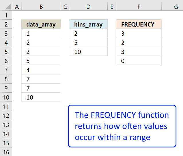
Returns how many times values exist in a given range. Note, this function returns an array of values.
Step 5 - Find first empty value (0) in array
MATCH(0, FREQUENCY(IF(EXACT($B$3:$B$15, TRANSPOSE($C$1:C1)), MATCH(ROW($B$3:$B$15), ROW($B$3:$B$15)), ""), MATCH(ROW($B$3:$B$15), ROW($B$3:$B$15))), 0)
returns 2.
Recommended articles
Identify the position of a value in an array.
Step 6 - Return value from position 2
INDEX($B$3:$B$15, MATCH(0, FREQUENCY(IF(EXACT($B$3:$B$15, TRANSPOSE($C$1:C1)), MATCH(ROW($B$3:$B$15), ROW($B$3:$B$15)), ""), MATCH(ROW($B$3:$B$15), ROW($B$3:$B$15))), 0))
returns "CC" in cell C3.
Recommended articles
Gets a value in a specific cell range based on a row and column number.
2.3 Excel file
Recommended articles
Case sensitive lookup and return multiple values
Filter values based on a condition - case sensitive (Excel 365)
Filter unique distinct values (case sensitive) [UDF]
Filter unique distinct records (case sensitive) [UDF]
3. Extract unique distinct values [Advanced Filter]
First a little reminder, unique distinct values are all cell values but duplicate values are merged into one distinct value.

3.1 Video
The following video shows you how to filter unique distinct values using Advanced Filter:
[adthrive-in-post-video-player video-id="Z61mnL2n" upload-date="2020-05-27T08:18:12.000Z" name="Filter unique distinct values using the Advanced Filter" description="How to extract unique distinct values using the Advanced Filter" player-type="default" override-embed="default"]
Subscribe to Get Digital Help on Youtube:
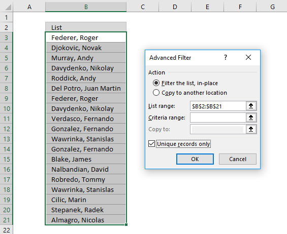
3.2 Instructions - Copy unique distinct values to another location

This section describes how to extract unique distinct values using the built-in feature "Advanced Filter".
- Go to tab "Data" on the ribbon.
- Press the "Advanced Filter" button on the ribbon.

- Press button "Copy to another location".

- Press "List range:" and select range to filter unique distinct values.
- Press "Copy to: and select a range.
- Press "Unique records only" button to select it.
- Press with left mouse button on "OK" button to apply settings and start extracting.

3.3 Instructions - Filter unique distinct values, in place
If you choose to filter unique distinct values in-place, press with left mouse button on the first option button in the dialog box.
You can then select unique distinct values and paste to another location, duplicate values are hidden and are ignored when you copy cell range B3:21 and paste to a new location, very useful.
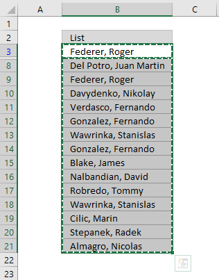
The picture below shows you the selected distinct values after I cleared the Advanced Filter, duplicate values are not selected because they were hidden.
Recommended articles
Lookup and return multiple values [Advanced Filter]
Extract all rows that meet critera in one column [Advanced Filter]
An Advanced Filter is not the only powerful built-in feature in Excel, I highly recommend that you learn pivot tables. Perhaps the most powerful tool but also the least known:
Recommended articles
A pivot table allows you to examine data more efficiently, it can summarize large amounts of data very quickly and is very easy to use.
The Excel defined table is also extremely useful, it allows you to quickly sort, filter and manipulate data. Learn that and much more:
Recommended articles
An Excel table allows you to easily sort, filter and sum values in a data set where values are related.
4. Highlight unique distinct values [Conditional Formatting]
This section demonstrates how to highlight unique distinct values using Excel's built-in feature "Conditional Formatting".
The image shows you unique distinct values highlighted using Conditional Formatting.
4.1 Video
This video demonstrates how to highlight unique distinct values:
[adthrive-in-post-video-player video-id="3yLRkWxc" upload-date="2020-05-27T08:34:12.000Z" name="Highlight unique values - Conditional Formatting" description="How to highlight unique distinct values using Conditional Formatting" player-type="default" override-embed="default"]
Subscribe to Get Digital Help on Youtube:
How to highlight unique distinct values
- Select cell range B3:B21.
- Go to tab "Home" on the ribbon.
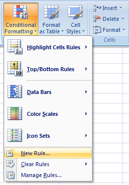
- Press on "Conditional Formatting" button.
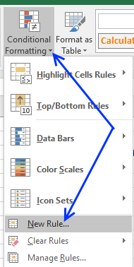
- Press on "New Rule...".
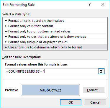
- Press on "Use a formula to determine which cells to format:".
- Type this formula: =COUNTIF($B$3:B3,B3)=1
- Press on "Format..." button.
- Pick a color.
- Press OK button.
- Press OK button again.
4.2 Explaining Conditional Formatting formula

A CF formula works somewhat differently than a regular formula, however, they may be harder to spot.
It is possible that you can't even see if a cell range has CF applied to it or not, if no cells are highlighted.
I recommend that you copy the CF formula and enter it to an adjacent column to better show how they work.
Step 1 - COUNTIF function
The COUNTIF function has two arguments, the first argument is the cell range you want to count a specific value in. The second argument is the value you want to count.
COUNTIF(range, criteria)
Step 2 - COUNTIF arguments
The first argument uses both relative and absolute cell references, $B$3:B3. The absolute part has dollar signs $B$3 meaning it does not change when the Conditional Formatting formula is applied to the next cell.
The relative part B3 does change when the Conditional Formatting formula is applied to the next cell.
COUNTIF($B$3:B3, B3)
Step 3 - Demonstrate calculations in cells B3 and B4
In cell B3 the function is COUNTIF($B$3:B3,B3)
and in cell B4: COUNTIF($B$3:B4,B4) and so on.
This technique using growing cell references lets you highlight the first instance of a value but not duplicate values.
Step 4 - Compare output to 1
How do we know if the value is a unique distinct value? Compare COUNTIF($B$3:B3,B3) to 1 and it will return TRUE or FALSE, like this:
COUNTIF($B$3:B3,B3)=1
The equal sign is a logical operator that returns TRUE or FALSE. Note, the comparison is not case sensitive. The output is a boolean value TRUE or FALSE.
COUNTIF($B$3:B3,B3)=1
becomes
1=1
and returns boolean value TRUE. Cell B3 is highlighted.
If COUNTIF($B$3:B3,B3) returns a number larger than 1 meaning there is at least a duplicate value in the cell range specified in the first argument. That prevents the Conditional Formatting formula from highlighting the cell.
Recommended articles
Highlight unique/duplicates
Highlight current date
Highlight lookup values
Highlight cells equal to
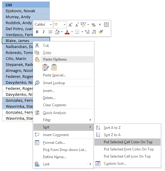
4.3 Sort Conditional formatted cells at the top
Tip! Press with right mouse button on on a highlighted cell, press with left mouse button on Sort and then on "Put Selected Cell Color On top" to arrange unique distinct values at the very top of your list.
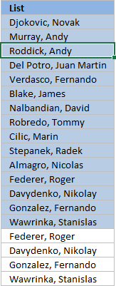
The picture below shows you all unique distinct values sorted together.
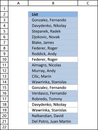
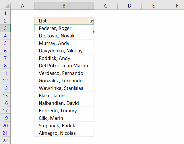
5. Hide duplicate values [Conditional Formatting]
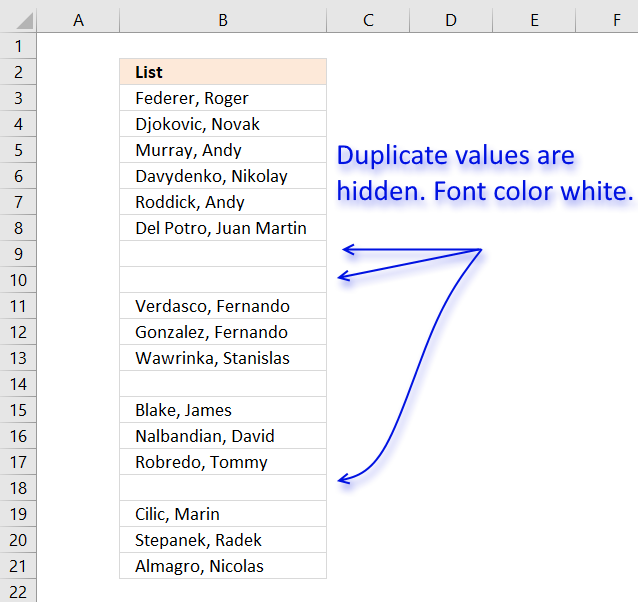
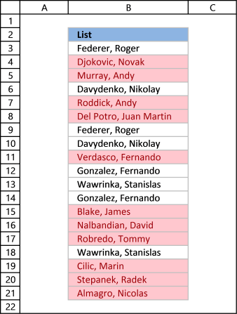
The image above demonstrates Conditional Formatting applied to a list of values, it changes the font color to white for duplicate values making them invisible or they appear hidden.
Keep in mind that the text is still there so if you copy the range and paste the values to a new range the hidden values are visible again. I recommend that you sort the visible values at the top in order to copy them correctly, instructions below.
Conditional Formatting formula:
How to apply conditional formatting formula to cell range B3:B21
- Select cell range B3:B21.
- Go to tab "Home" on the ribbon.
- Press with left mouse button on the "Conditional Formatting" button.
- Press with left mouse button on "New Rule..."
- Press with left mouse button on "Use a formula to determine which cells to format:".
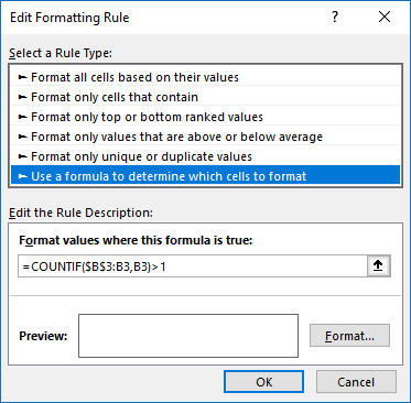
- Type the Conditional Formatting formula in "Format values where this is true:".
- Press with left mouse button on "Format..." button.
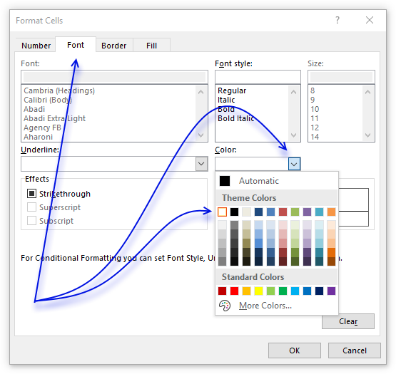
- Go to tab "Font" on the menu, see image above.
- Press with left mouse button on color drop-down list.
- Pick white.
- Press with left mouse button on OK button.
- Press with left mouse button on OK button.
- Press with left mouse button on OK button.
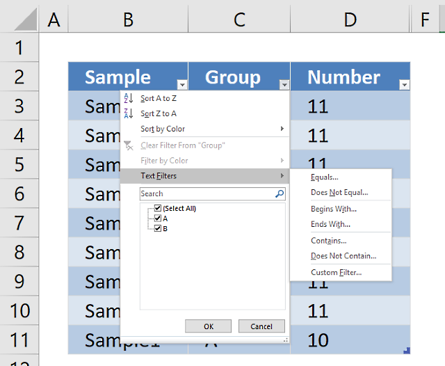
6. How to sort unique distinct values at the top of the list
- Press with right mouse button on on one of the visible values in the list.
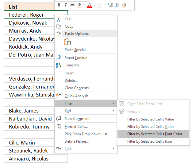
- Press with left mouse button on "Filter"
- Press with left mouse button on "Filter by Selected Cell's Font color.
Recommended articles
Highlight unique values and unique distinct values in a multi-column cell range
Highlight unique distinct records
Highlight unique values in a filtered excel table
How to highlight duplicate values in a column
Check out the Conditional formatting category
7. Extract unique distinct sorted values from a cell range [UDF]

This UDF lets you create and sort a unique distinct list. First you need to copy the VBA code to your workbook, instructions below. Second, select a cell range. Third, type FilterUniqueSort(cell_ref) in the formula bar. Last, enter formula as an array formula, instructions below.
There is also a workbook for you to get.
Array formula in cell B2:B8212:
7.1 Video
This video explains how to implement and use the User Defined Function
[adthrive-in-post-video-player video-id="hO4E5kV4" upload-date="2020-05-27T08:58:13.000Z" name="Extract unique distinct values sorted from A to Z no blanks UDF" description="Extract unique distinct values sorted from A to Z no blanks UDF" player-type="default" override-embed="default"]
Subscribe to Get Digital Help on Youtube:
7.2 How to create an array formula
- Type B2:B8212 in name box
- Type above array formula in formula bar

- Press and hold Ctrl + Shift
- Press Enter once
- Release all keys
Recommended reading
Recommended articles

Array formulas allows you to do advanced calculations not possible with regular formulas.
7.3 VBA code
I am using the selection sort function to sort values. You can read more about the function here:
Using a Visual Basic Macro to Sort Arrays in Microsoft Excel
'Name User Defined Function and define paremeter
Function FilterUniqueSort(rng As Range)

'Dimension variables and declare data types
Dim ucoll As New Collection, Value As Variant, temp() As Variant
Dim iRows As Single, i As Single

'Redimension array variable
ReDim temp(0)

'Enable error handling
On Error Resume Next

'Iterate through each value in range
For Each Value In rng

'Check if number of characters in value is greater than 0 (zero), if true add value to collection ucoll
If Len(Value) > 0 Then ucoll.Add Value, CStr(Value)

'Continue with next value
Next Value

'Disable error handling
On Error GoTo 0

'Iterate through each value in collection ucoll
For Each Value In ucoll

'Save value to last container in array variable temp
temp(UBound(temp)) = Value

'Add new container to array variable temp
ReDim Preserve temp(UBound(temp) + 1)

'Next value
Next Value

'Remove last container in array variable temp
ReDim Preserve temp(UBound(temp) - 1)

'Save selected rows on worksheet to variable iRows
iRows = Range(Application.Caller.Address).Rows.Count

'Start User Defined Function SelectionSort with values in array variable temp
SelectionSort temp

'Add blanks to array variable temp to prevent error values on worksheet
For i = UBound(temp) To iRows

'Add container
ReDim Preserve temp(UBound(temp) + 1)

'Save blank to container
temp(UBound(temp)) = ""

'Continue with next value
Next i

'Transpose values in array variable temp and return those values to worksheet
FilterUniqueSort = Application.Transpose(temp)

End Function
'Name User Defined Function (UDF) and define parameters
Function SelectionSort(TempArray As Variant)
'This UDF sorts values in an array
'https://www.get-digital-help.com/how-to-extract-a-unique-list-and-the-duplicates-in-excel-from-one-column/#7.3

          'Dimension variables and declare data types
          Dim MaxVal As Variant
          Dim MaxIndex As Integer
          Dim i As Integer, j As Integer

          'Iterate through each value in array variable temp starting from last to first
          For i = UBound(TempArray) To 0 Step -1

              'Save value to variable MaxVal
              MaxVal = TempArray(i)

              'Save value stored in variable i to variable MaxIndex
              MaxIndex = i

              'Iterate through each value in array variable temp
              For j = 0 To i

                  'Check if value in array variable TempArray is larger than value stored in variable MaxVal
                  'Excel can compare text values as well, this action checks if a text value is before or after another value in a sorted list
                  If TempArray(j) > MaxVal Then

                      'If true save value to variable MaxVal
                      MaxVal = TempArray(j)

                      'Save position to MaxIndex
                      MaxIndex = j
                  End If

              'Continue with next value
              Next j

              'Check if number stored in variable MaxIndex is smaller than number stored in variable i
              If MaxIndex < i Then

                  'Save value in array variable TempArray position i to array variable TempArray container position MaxIndex
                  TempArray(MaxIndex) = TempArray(i)

                  'Save value in variable MaxVal to array variable TempArray container position i
                  TempArray(i) = MaxVal
              End If
          Next i

      End Function
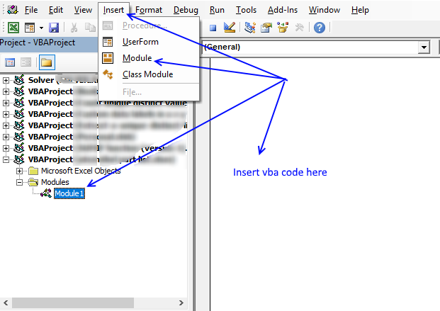
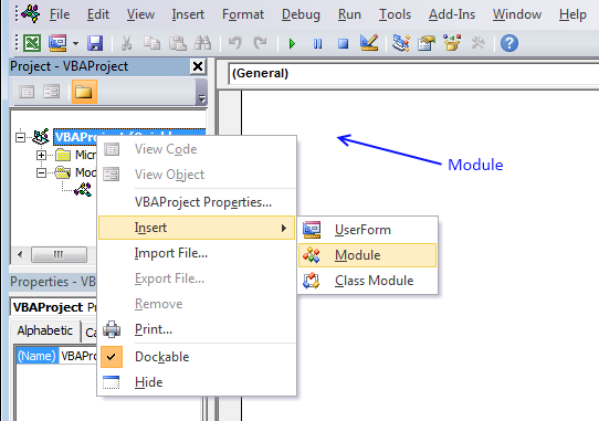
7.4 Where to copy VBA code?
- Press Alt + F11 to open VB Editor
- Press with left mouse button on "Insert" on the menu
- Press with left mouse button on "Module" to create a module
- Copy (Ctrl + c) above VBA code and paste (Ctrl +v) to the code module
More powerful User Defined Functions
Recommended articles
This article demonstrates two ways to extract unique and unique distinct rows from a given cell range. The first one […]
Recommended articles
This article demonstrates how to find a value in a column and concatenate corresponding values on the same row. The […]
Recommended articles
This blog post describes how to create a list of unique distinct words from a cell range. Unique distinct words […]
8. Filter unique distinct values from multiple sheets add-in
Filter unique distinct values is an add-in for Excel 2007/2010/2013 that lets you extract
- unique distinct values
- duplicate values
- unique distinct records
- duplicate records
from multiple sheets. The Add-In contains 4 user-defined functions.
If a value in one of the ranges changes the function will automatically and instantly update the list.
Features
- All user-defined functions remove blank values and blank records.
- No error values when all values are extracted.
- Filter values or records from up to 255 different cell ranges or sheets.
8.1 Watch this video where I demonstrate the Excel Add-In
![]()
Subscribe to Get Digital Help on Youtube:
What are unique distinct values?

What are unique distinct records?

Purchase Filter Unique Distinct Values From Multiple Sheets Add-in For Excel 2007/2010/2013 - Price $19 USD


![]()
![]()

Questions
Is there a money back guarantee?
Sure, you have a unconditional money back guarantee for 14 days.
9. Create a list of unique distinct values [Old array Formula]
I recommend using the regular formula above since it is smaller and has an advantage of not being an array formula.
Array formula in cell D3:
Thanks to Eero, who contributed the original array formula!
The formulas above has an issue with blank cells, it returns a 0 (zero) in your list. This article shows you how to ignore blanks:
Recommended articles
This article demonstrates formulas that extract unique distinct values and ignore blank empty cells. Table of contents Extract a unique […]
9.1 How to create an array formula
You don't need to follow these steps if you chose the regular formula.
- Copy the array formula above (Ctrl + c)
- Double press with left mouse button on cell B2
- Paste (Ctrl + v)
- Press and hold Ctrl + Shift simultaneously
- Press Enter
- Release all keys
If you made the above steps correctly the formula now has a beginning and ending curly bracket, like this:
{=INDEX($B$3:$B$21, MATCH(0, $D$2:D2, $B$3:$B$21), 0))}
Don't enter these characters yourself, they appear automatically.
Copy cell B2 and paste to cells below as far as needed.
9.2 How the array formula in cell B2 works
Step 1 - Create an array with the same size as the list
The COUNTIF function calculates the number of cells equal to a condition.
COUNTIF(range, criteria)
COUNTIF($B$1:B1, $A$2:$A$20)
returns:
{0;0;0;... ;0}
This means the cell value in $B$1:B1 can't be found in any of the cells in cell range $A$2:$A$20. If it had been found, somewhere in the array the number 1 would exist.
Step 2 - Return the position of an item that matches 0 (zero)
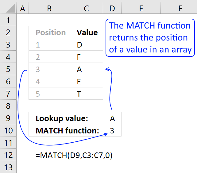
The MATCH function returns the relative position of an item in an array that matches a specified value.
MATCH(lookup_value, lookup_array, [match_type]
MATCH(0, COUNTIF($B$1:B1, $A$2:$A$20), 0)
eturns 1.
Step 3 - Return a cell value
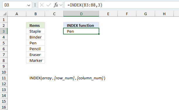
The INDEX function returns a value or reference of the cell at the intersection of a particular row and column, in a given range.
INDEX(array, row_num, [column_num])
INDEX($B$3:$B$21, 1)
returns "Federer, Roger".
Relative and absolute cell references
When you copy the array formula down the countif formula range ($B$1:B1) expands. This is created by using relative and absolute references.
The first cell, B2: COUNTIF($B$1:B1,$A$2:$A$20)
Second cell, B3: COUNTIF($B$1:B2,$A$2:$A$20)
and so on.
Recommended reading:
Recommended articles
What is a reference in Excel? Excel has an A1 reference style meaning columns are named letters A to XFD […]
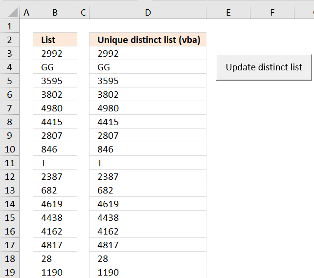
10. Create a unique distinct list using Advanced Filter in a macro
Question:
A comment from this blog post: How to extract a unique distinct list of a column in excel
Answer: I created a random list of 5000 values. Creating a unique distinct list using Advanced Filter only took a couple of seconds. Maybe that is fast enough?
I also tried sorting the list and using MATCH() (which is fast) to filter unique distinct values but that required a lot of manual work. Maybe someone else have some lightning fast formula technique?
I then created a macro, recording my actions using Advanced Filter. I edited the vba code and inserted a button (Form Control). How to Run an Excel Macro With a Worksheet Button
Press with left mouse button oning the button refreshes the unique distinct list. Adding values to the list is no problem, the selection extends as long as there are no blank cells.

How to automatically use Advanced Filter to create a unique distinct list
- Press with left mouse button on "Developer" tab How to show the Developer tab or run in developer mode
- Press with left mouse button on "Visual Basic"
- Create a "Module" for your workbook How to Copy Excel VBA Code to a Regular Module
- Copy this vba code into module:
Sub AdvFilter() '
' AdvFilter Macro

' Select first cell in column (Sheet1!A2)
Range("Sheet1!A2").Select

' Extending the selection down to the cell just above the first blank cell in this column
Range(Selection, Selection.End(xlDown)).Select

' Run Advanced Filter on selection and copy to Sheet1!C2
Selection.AdvancedFilter Action:=xlFilterCopy, CopyToRange:=Range( _ "Sheet1!C2"), Unique:=True End Sub
Assign macro to button
How to Run an Excel Macro With a Worksheet Button
Get excel sample file for this tutorial.
Remember to enable macros.
quick unique distinct list.xls
(Excel 97-2003 Workbook *.xls)
11. Filter unique distinct values - case sensitive - UDF
The User Defined Function demonstrated in the above picture extracts unique distinct values also considering lower and upper case letters.
There are now Excel 365 formulas that creates this task:
- Filter unique distinct rows case sensitive - Excel 365 recursive LAMBDA function
- Count unique distinct rows case sensitive
A User defined Function in Excel is a custom function that anyone can use, simply copy the code to your workbook and you are good to go, see details below.
Array formula in cell D3:D10:
To enter an array formula, type the formula in a cell then press and hold CTRL + SHIFT simultaneously, now press Enter once. Release all keys.
The formula bar now shows the formula with a beginning and ending curly bracket telling you that you entered the formula successfully. Don't enter the curly brackets yourself.
Have you read the article that extracts unique distinct values (case sensitive) using an array formula?
User defined Function Syntax
CSUnique(rng)
Arguments
| Parameter | Text |
| rng | Required. The range you want to use. |
VBA
'Name function and argument
Function CSUnique(rng As Range)
'Declare variables and data types
Dim cell As Range, temp() As String, i As Single, iRows As Integer
'Redimension array variable so it can grow using Redim Preserve statement
ReDim temp(0)
'Iterate through each cell in range
For Each cell In rng
  'Iterate through values in array variable temp
  For i = LBound(temp) To UBound(temp)
    'If value is equal to cell value
    If temp(i) = cell Then
       'Add one to variable i
       i = i + 1
       'Stop For ... Next statement
       Exit For
    End If
  Next i
  'Subtract variable i with 1
  i = i - 1
  'If value in array variable temp is not equal to cell value
  If temp(i) <> cell Then
    'Save cell value to array variable temp
    temp(UBound(temp)) = cell
    'Add another container to array variable temp
    ReDim Preserve temp(UBound(temp) + 1)
  End If
Next cell
'Count how many cells have been used when entering UDF
iRows = Range(Application.Caller.Address).Rows.Count
'To prevent error value the UDF adds blanks to remaining containers
If iRows < UBound(temp) Then
  temp(iRows - 1) = "More values.."
Else
  For i = UBound(temp) To iRows
    ReDim Preserve temp(UBound(temp) + 1)
    temp(UBound(temp)) = ""
  Next i
End If
'Return array variable temp to worksheet
CSUnique = Application.Transpose(temp)
End Function
End Function
Where to copy vba code?
- Press Alt-F11 to open visual basic editor
- Press with right mouse button on on your workbook in 'Project Explorer' window
- Press with left mouse button on 'Insert'
- Press with left mouse button on 'Module'
- Copy above VBA code
- Paste VBA code to the code module
- Exit visual basic editor
12. How to filter unique values from a list

Unique values are values existing only once in a list. Example, "AA" exists twice in the list below and is not unique. BB and CC exist only once each and are unique in the list.
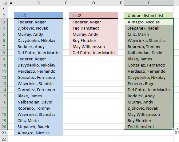
Column D in the picture below filters all unique values from column B. Unique values are values that exist only once in column B.

Example, Roger, Federer is not in column D because there is more than one value of this name in column A. In other words, the name is not unique in column A. You can find the name twice in the list, in cells A2 and A8.
Update 2017-08-30
This formula is even smaller than the array formula and you are not required to enter this as an array formula.
Regular formula in cell D3:
Recommended articles
How to extract a case sensitive unique list from a column
Filter unique values sorted from A to Z
Extract unique values from two columns
Update 2020-12-09, the formula below extracts unique values from cell range $B$3:$B$21:
Regular formula in cell D3:
The formula above contains the new UNIQUE function that only Excel 365 subscribers can use. Use the formula above if you have an earlier Excel version.
Recommended articles
Extract unique values - Excel 365 (Link)
Extract unique values sorted from A to Z - Excel 365 (Link)
Extract unique values ignoring blanks - Excel 365 (Link)
Extract unique values sorted from A to Z ignoring blanks - Excel 365 (Link)
Array formula in cell D3:
12.1 Explaining array formula in cell D3
Step 1 - Count each value in array and check if it is not equal to one
(COUNTIF($A$2:$A$20, $A$2:$A$20)<>1
returns
{TRUE; FALSE; FALSE; ...; FALSE}
This array tells excel that the first value in the array is not unique and that is true because Roger, Federer is not unique in the list. However the second value is FALSE and that value is unique, etc.
Recommended articles
Counts the number of cells that meet a specific condition.
Step 2 - Keep track of previous values
C1:$C$1 is a dynamic cell reference, it changes as the formula is copied to cells below. You can read more about absolute and relative cell references here:
Recommended articles
What is a reference in Excel? Excel has an A1 reference style meaning columns are named letters A to XFD […]
COUNTIF(C1:$C$1, $A$2:$A$20)
returns
{0; 0; 0; ... ; 0}
A zero (0) means that no values have yet been displayed and that is true in cell C2. However when excel calculates the value in cell C3, cell C2 shows "Djokovic, Novak" and the array becomes {0; 1; 0; ... ; 0}. The second value in the array contains 1. This tells excel that value has already been shown.
Step 3 - Add arrays
COUNTIF(C1:$C$1, $A$2:$A$20)+(COUNTIF($A$2:$A$20, $A$2:$A$20)<>1
returns
{1;0;0;... ;0}
TRUE is 1 and FALSE is zero. So True + 0 equals 1 and False + 1 equals 1.
Step 4 - Find first zero value in array
A zero in the array indicates {1;0;0;1;0;0;1;1;0;1;1;1;0;0;0;1;0;0;0} that the corresponding value is unique and has not yet been displayed in the list.
MATCH(0, COUNTIF(C1:$C$1, $A$2:$A$20)+(COUNTIF($A$2:$A$20, $A$2:$A$20)<>1), 0)
returns 2.
Step 5 - Return corresponding value
INDEX($A$2:$A$20, MATCH(0, COUNTIF(C1:$C$1, $A$2:$A$20)+(COUNTIF($A$2:$A$20, $A$2:$A$20)<>1), 0))
returns "Djokovic, Novak" in cell C2.
11.2 Get Excel file
To extract duplicates, see this post:
Recommended articles
The array formula in cell C2 extracts duplicate values from column A. Only one duplicate of each value is displayed […]
13. Highlight unique values [Conditional Formatting]
This example demonstrates how to highlight cells with a color of your choice if it contains a unique value.
12.1 Video
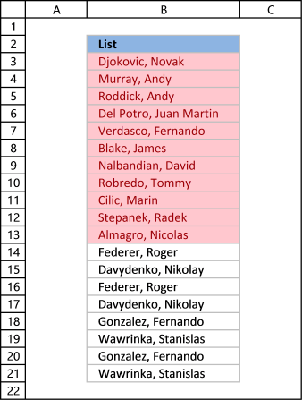
The following video shows you how to color unique values using conditional formatting. Remember, it highlights only unique values, in other words, values that exist only once in the list.
[adthrive-in-post-video-player video-id="3yLRkWxc" upload-date="2020-05-27T08:34:12.000Z" name="Highlight unique values - Conditional Formatting" description="How to highlight unique distinct values using Conditional Formatting" player-type="default" override-embed="default"]
Subscribe to Get Digital Help on Youtube:
Instructions
- Go to tab "Home" on the ribbon
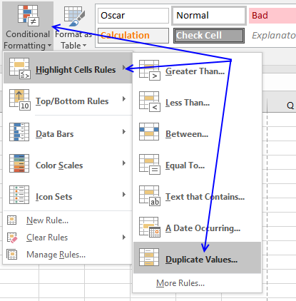
- Press with left mouse button on "Conditional Formatting" button
- Hover over "Highlight Cell Rules"
- Press with mouse on "Duplicate Values..."
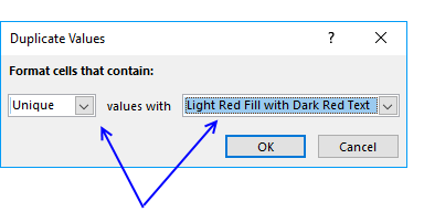
- Press with mouse on the leftmost drop-down list and change it to "Unique"
- Pick a formatting if you like
- Press with left mouse button on OK button
The picture above shows you, for example, that the first name in the list has a duplicate so that name is not highlighted in any cell.
13.2 Sort unique values at the top
Tip! Did you know that you can put highlighted values to the top
- Press with right mouse button on on a highlighted cell
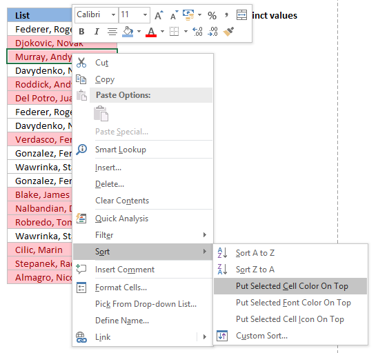
- Press with mouse on "Sort"
- Press with mouse on "Put Selected Cell Color On Top"
14. Useful tips
14.1 Excel tables
An Excel Table is a great feature and is very cleverly designed. It is constructed to automatically expand if you add more data which is incredibly helpful. You don't need to do anything, not adjusting cell references which is time consuming and prone to errors.
Structured references are cell references to an excel defined table. They let you easily see what the data contains as long as you give it good descriptive column header names.
I recommend you use excel defined tables instead of named ranges or dynamic named ranges as long as you are working with more than one value.
Here is how to convert a list to an excel defined table:
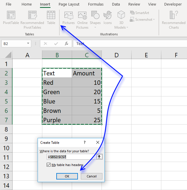
- Select a cell in your list
- Go to tab "Insert" on the ribbon and press with left mouse button on Table button or press Ctrl + T
- Press with left mouse button on OK button
- Your excel defined table is created
Read more about excel defined tables
14.2 Named ranges
In excel you can name a cell range, a constant or a formula. You can then use the named range in a formula, making it easier for you to read and understand formulas.
Example
List : A2:A20
Tip! Use dynamic named ranges to automatically adjust cell ranges when new values are added or removed.
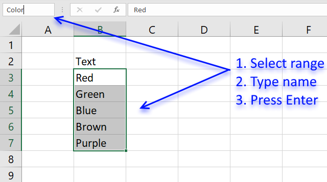
14.2.1 How to create a named range
The downside with named ranges is that you need to adjust the range every time you add or delete a value in the list, the named range will then not fit the value list. I recommend using excel defined tables if you know that the list may change in the future.
- Select cell range B3:B7
- Type Color in name box
- Press Enter
Formula example containing name range:
15. How to remove errors (Excel 2007)
Excel 2007 users (and later versions) can remove errors using IFERROR() function.
When the formula runs out of values it returns #N/A errors (Not Available), you can use the IFERROR function to remove the error and return blanks in those cells.
Unfortunately, it comes with a big disadvantage, it also removes other formula errors as well. So use this with great caution. If your source table has errors you won't detect it because the IFERROR function returns a blank cell instead.
Array formula in cell D2:
and copy it down as far as necessary.
Recommended articles
How to use the IFERROR function
How to use the ISERROR function
How to use the ERROR.TYPE function
How to find errors in a worksheet
Delete blanks and errors in a list
16. Excel 2003 users can remove errors using isna() function:
and copy it down as far as needed.
This formula is an array formula, how to enter an array formula.
Recommended article
17. How to ignore blank cells in a range
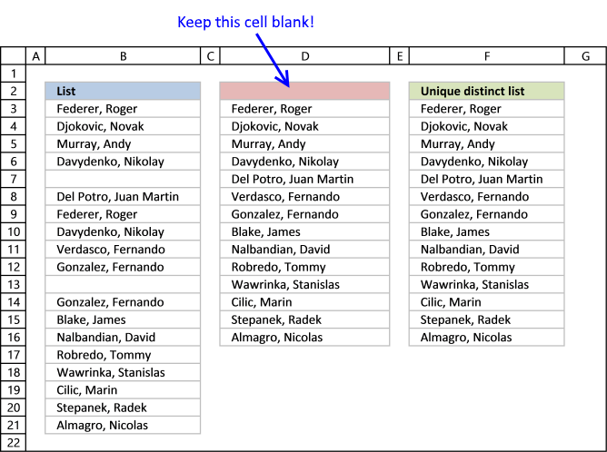
Harlan Grove created a formula to count unique distinct values from a list with blanks. I used the same technique here to filter unique distinct values in column D.
If you want a header name you can use the slightly larger formula, displayed in column F below.
Update 2020-12-09, Excel 365 users can use this regular formula:
The formula below is actually 58 character while the new Excel 365 formula above is 61 characters, space characters not included. You can find a formula explanation here: Extract unique distinct values ignoring blanks
Use the formula below if you have an earlier Excel version than Excel 365.
Update 2017-09-01, smaller regular formula in cell D3:
Formula in cell F3 if you need a column header name:
16.1 Watch a video where I explain how these two formulas work
[adthrive-in-post-video-player video-id="ba63YnWm" upload-date="2020-05-27T07:37:09.000Z" name="Extract unique distinct values ignore blanks" description="How to extract a unique distinct list ignoring blanks using a formula" player-type="default" override-embed="default"]
This article shows you how to fill blank cells with values or formulas
Recommended articles
Learn how to extract non-blank cells in a list using a formula:
Recommended articles
In this blog post I will demonstrate methods on how to find, select, and deleting blank cells and errors. Why […]
16.2 Get Excel file
Advanced filter excel category
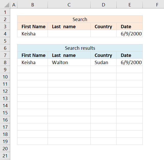
This article demonstrates a formula that allows you to search a data set using any number of conditions, however, one […]
Unique distinct values category
This article demonstrates Excel formulas that allows you to list unique distinct values from a single column and sort them […]
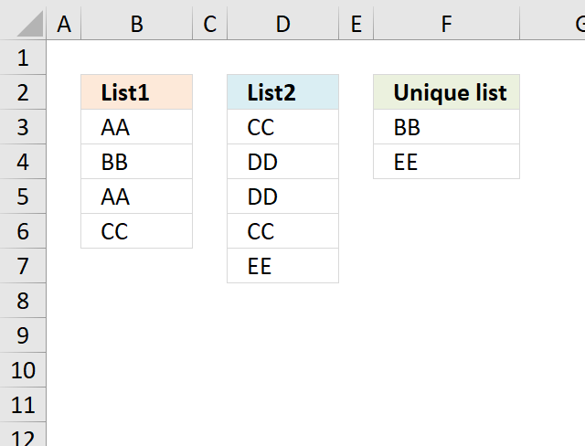
Question: I have two ranges or lists (List1 and List2) from where I would like to extract a unique distinct […]
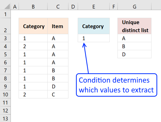
This article shows how to extract unique distinct values based on a condition applied to an adjacent column using formulas. […]
Unique values category
What's on this page Extract unique values from two columns - Excel 365 Extract unique values from two columns - […]
Excel categories
165 Responses to “5 easy ways to extract Unique Distinct Values”
How to comment
How to add a formula to your comment
<code>Insert your formula here.</code>
Convert less than and larger than signs
Use html character entities instead of less than and larger than signs.
< becomes < and > becomes >
How to add VBA code to your comment
[vb 1="vbnet" language=","]
Put your VBA code here.
[/vb]
How to add a picture to your comment:
Upload picture to postimage.org or imgur
Paste image link to your comment.
Hey there - thanks a lot for this tip - though I initially could not get this to work - eventually I figured out MY problem the INDEX rownum was using "ROW(A2:A20)-1", when it should be using "ROW()-1" - otherwise it ALWAYS returns the start of the array.
Thank you for visiting Get Digital Help and commenting! I have changed the formula and the attached file. Using named ranges simplifies formula customization a lot!
Many thanks for the useful information posted on this website! However, as I am working on a very large set of data (from between 50 - 8000 records) and whenever I change the name range to go beyond the 1000th record, the unique list value would return error. I have tried to name the whole column A but it also doesnt work.
would be grateful if you could assist on this.
Many thanks for all your effort!
Thank you!
I tried to recreate your error, but failed. I have attached an excel file with over a 1000 records that works for me. The excel file is at the end of the above blog post. Try it and see if the excel file returns an error.
I am using excel 2007, what version are you using?
Have you changed cell ranges for both named ranges in your excel sheet?
List (A2:A20)
unique_start (B2)
Maybe you have a blank cell somewhere in your list? A blank cell returns an error. See this post:
https://www.get-digital-help.com/how-to-automatically-create-a-unique-list-and-remove-blanks/
There is a somewhat shorter approach:
Let initial items in colA be named as "List". In B2 enter the
following array-formula:
=INDEX(List,MATCH(0,COUNTIF($B$1:B1,List),0)) and copy it down as far as necessary, to get unique list.
That is really amazing, you made the array formula even shorter!
To remove any errors, Excel 2007 users can use IFFERROR() function:
=IFERROR(INDEX(List,MATCH(0,COUNTIF($B$1:B1,List),0)),"") + CTRL + SHIFT + ENTER and copy it down as far as necessary.
Thank you for your valueable comment!
hi.
thanks for the formulas (eero's and the revised one) guys. it really cured my headaches.
for the unique list generated (Column B), can the...
1) unique list sorted A-Z order?
2) unique list sorted based on occurrence (highest to lowest)?
the trick is: can the sorting be done without complicating eero's formula above?
reason i'm asking because the other posts on sorting is too complicated for my head to wrap around ;)
thx!
Interesting questions!
I´ll see if I can come up with some good solutions.
Thanks for commenting!
thanks!
in case you're wondering, eero's formula does not need the unique list range (Column B) to be same size as the main list (Column A).
I just need to copy down the formula to get the rest of the unique list.
Your other posts on sorting is based on range-based array formula (i.e. Column B must be same size as Column A in order for the array formula to work). This works well if you have short list, but if u have thousands of entries, unique list range must equal the same.
One other that thing that i noticed is the ranged-based array formula is fixed (you can't delete those 'empty' cells in this range).
anyways, thanks again for looking into another solutions and not to forget your valuable blogs here!
David, here is the answer to your first question.
unique list sorted A-Z order?
Array formula in cell B2, see picture above.
=INDEX(List, MATCH(MIN(IF(COUNTIF($B$1:B1, List)=0, 1, MAX((COUNTIF(List, "<"&List)+1)*2))*(COUNTIF(List, "<"&List)+1)), COUNTIF(List, "<"&List)+1, 0)) + CTRL + SHIFT + ENTER and copy it down as far as necessary, to get unique list sorted alphabetically from A to Z. If anyone can come up with a shorter formula, i would be happy!
oh wow! it works! :)
THANKS!
David, here is the answer to your second question.
unique list sorted based on occurrence (highest to lowest)?
Array formula in cell B2, see picture above.
=INDEX(List, MATCH(IF(MAX(COUNTIF(List, List)*IF(COUNTIF(B$1:$B1, List)=1, 0, 1))=0, 1, MAX(COUNTIF(List, List)*IF(COUNTIF(B$1:$B1, List)=1, 0, 1))), COUNTIF(List, List)*IF(COUNTIF(B$1:$B1, List)=1, 0, 1), 0))+ CTRL + SHIFT + ENTER and copy it down as far as necessary, to get sorted based on occurrence (highest to lowest)
I have to think some more to get this formula shorter, I don´t like the length of it.
works great! :D
thanks!
p/s: as long as the array formula works, i'm happy. but do keep up your great job on the formulas! MS Excel gurus should visit and give you a thumbs up! :)
Wow the short formula works, amazing!!!
Thanks!
Wow! This is just amazing. Works great. I would love if someone could explain how this works step by step. I tried, but couldn't. I am trying to extend this fomula with a user defined formula.
[...] How to extract a unique distinct list from a column in excel [...]
Sriram Venkitachalam,
I now have tried to explain the array formula, see the new section above.
Thanks for commenting!
Would you please advise me on how to created named range which includes A-Z sorted list of UNIQUE values of other list?
Thanks a lot for this example. But is there also a way without using CSE? because a use a tool where i import Excel file which does not support CSE formulas in Excel.
Hopefuly someone has an idea
Dear All, It's my first post right here, and I'd like to thank you all with special THANKS for ADMIN. Well, I'm looking for more info and explanation about the current topic of https://www.get-digital-help.com/how-to-extract-a-unique-list-and-the-duplicates-in-excel-from-one-column/ It has mentioned above,
"How this array formula works: =INDEX(List,MATCH(0,COUNTIF($B$1:B1,List),0)) The array formula uses MATCH() to find the first 0 (zero) value in the COUNTIF array. When you copy the array formula down the COUNTIF formula range expands. The first cell: COUNTIF($B$1:B1,List), the second cell: COUNTIF($B$1:B2,List) and so on"
It's understood, but I'm still puzzled for the following reasons:
1. When applying the mentioned formula, the result is always the first record only.
2. All array elements shows INDEX(List,MATCH(0,COUNTIF($B$1:B1,List),0)) in formula bar, which indicates that the range expansion mentioned above is not applicable.
3. The attached example sheet shows
@ cell B2: INDEX(List,MATCH(0,COUNTIF(B1:$B$1,List),0)),
while @ cell B3: INDEX(List,MATCH(0,COUNTIF(B$1:$B2,List),0)),
and It’s OK, if we are talking about singular cell formula.
So how come (B1:$B$x) changed into (B$1:$Bx) from cell to another within the same array command?
Do I miss something?
Is there any Excel settings should be takes place?
Please help & advise.
Thank YOU & BEST Regards,
Raymond,
You need to convert your formulas to values.
Copy and "Paste Special.." the values created by the CSE formula.
Select "Values" and press with left mouse button on OK button.
OnlineAlone,
Copy =INDEX(List,MATCH(0,COUNTIF($B$1:B1,List),0)) + CTRL + SHIFT + ENTER into your first cell. (Cell B2)
Copy your first cell an paste to the remaining cells.
The formula then automatically changes to:
Cell B3: =INDEX(List,MATCH(0,COUNTIF($B$1:B2,List),0))
Cell B4: =INDEX(List,MATCH(0,COUNTIF($B$1:B3,List),0))
and so on.
Oscar,
Thank you for your quick response.
OK, I got it.
OnlineAlone,
I missed this question:
So how come (B1:$B$x) changed into (B$1:$Bx) from cell to another within the same array command?
You have found an error in the attached file.
I have now changed the formula in the attached file and uploaded it to this blog post again.
Here is an excellent explanation of absolute and relative references:
https://www.cpearson.com/excel/relative.aspx
hi all,
thanks for the great formula/array formula. it works great.
lately, i noticed that the array formula will make the excel calculations CRAWL if I have thousands of entries (dates; but mostly repeated because of different product).
e.g.
1-Jan-2010 ProductA
1-Jan-2010 ProductB
1-Jan-2010 ProductC
1-Jan-2010 ProductD
2-Jan-2010 ProductA
2-Jan-2010 ProductB
2-Jan-2010 ProductC
...
...
the unique distinct values from the dates are 1-Jan-2010, 2-Jan-2010, and so on.
In a month (31-days) x 13 products = 403 entries. Multiply this to 12-months = 403 x 12 months ~est. 4.9k dates to be parsed.
the jackpot question: Is there a way to easily parse long list, without sacrificing performance (recalculations)?
thx!
David,
have you tried "Advanced Filter"?
https://www.get-digital-help.com/how-to-extract-a-unique-list-and-the-duplicates-in-excel-from-one-column/#advfilter
Thanks for commenting!
2 problems i see using Advanced Filter:
a) The first 2 generated entry is a repeat. i.e. 1-Jan-2010, 1-Jan-2010, 2-Jan-2010, 3-Jan-2010, and so on.
first entry is named “Extract”).
b) The dates from my master table is set with a dynamic named range. Advanced Filter will generated unique
distinct list, manually.
I daily update the table
thx!
david,
See this blog post (and the attached file):
https://www.get-digital-help.com/create-a-unique-distinct-list-of-a-long-list-without-sacrificing-performance-using-vba-in-excel/
just noticed this standalone post. incredible.
will try it out.
note: reason why Advance Filter is not preferred (by me anyway) is the list will gets longer daily. i wouldn't want to keep (manually) using Advanced Filter.
'sides, i'm preparing the file for Excel noobs. he/she should not be complicated by the steps :D
the VBA macro button is interesting tho! will try it now!!
thx guys!!
hi oscar, finally been trying very hard to use this. my situation as such:
1) First sheet is called VC (the master table with dates).
2) Second sheet is called Calc (where the calculations are located).
3) Third sheet is called Charts (where the VBA-macro button is located).
Charts sheet is the only visible sheet. Managers are viewing this only.
Calc sheet is hidden (to prevent ppl snooping or ruin the formulas :))
It seems that Advanced Filter function itself cannot PUSH filtered data to Calc sheet (target).
I've tried the other way round to PULL filtered data from VC sheet (source). However, the macro uses an absolute address of the selected range.
this is the vb code in Calc sheet:
Sub Macro3()
'
' Macro3 Macro
'
'
Sheets("VC").Range("A2:A5004").AdvancedFilter Action:=xlFilterCopy, _
CopyToRange:=Range("C2"), Unique:=True
End Sub
David, try this:
Sub AdvFilter()
'
' AdvFilter Macro
Range("VC!A2").Select
Range(Selection, Selection.End(xlDown)).Select
Selection.AdvancedFilter Action:=xlFilterCopy, CopyToRange:=Range( _
"Calc!C2"), Unique:=True
End Sub
thx oscar. it works, but only after i added this:
Sub AdvFilter()
'
' AdvFilter Macro
Sheets("VC").Select
Range("VC!A2").Select
Range(Selection, Selection.End(xlDown)).Select
Selection.AdvancedFilter Action:=xlFilterCopy, CopyToRange:=Range( _
"Calc!C2"), Unique:=True
Sheets("Chart").Select
End Sub
-----------
problem with Adv Filter is that it cant just pull data from another sheet. The sheet must be active before Adv Filter can be executed.
my rough tweak is to Select the VC sheet first, then let the Adv Filter routine run (generated on Calc sheet). Then change back to Chart sheet where the button is.
this creates a short sheet "flipping" when the button is created.
David,
To remove "flipping" use: Application.ScreenUpdating = False
/Oscar
thx oscar, the "no-flipping" function works.
btw, do u know that the Adv Filter-unique value doesnt work if the first 2 values are the same?
e.g.
10001
10001
10001
10002
10002
10003
10004
10004
10005
generated list from Adv Filter are...
10001 <-repeat
10001 <-repeat
10002
10003
10004
10005
david,
Advanced Filter uses your first value as a column header.
/Oscar
I been trying to do this for a long time. I tried by pivotTable to extract the list without duplicate items.
This much easier, clear, and great! Thanks a lot!
I found out the column 'A' must choose the title of it 'A1' also, to avoid in column 'B' shows 'A2' twice, and there is no problem to choose 'A1' coz it shows the same title in 'B1'.
Thanks again!
In excel 2003 and older you can remove error by using ISNA() function.
The formula is brilliant but it took me some significant amount of time to understand it (use Evaluate formula).
Wiciu,
Thanks!! I have added the ISNA() function to this post.
/Oscar
Oscar, these countif function formulas are great because they are able to extract a list with blank cells in the range. Is there a way to extract a list using sum(if instead of countif because this will work with closed workbooks (when the need arises), while also having the ability like the countif function to handle blank cells in the range? Maybe we need to put a condition in the front of the formula to handle the blank cells. Keep up the brilliant work. This website is one of the top Excel websites out there.
Sean,
Thanks!
As far as I know, you can´t extract a unique distinct list from a closed workbook with excel formulae.
Sean,
See this post: https://www.get-digital-help.com/extract-unique-distinct-numbers-from-closed-workbook-in-excel-formula/
Sean,
Here is another post: https://www.get-digital-help.com/extracting-unique-distinct-text-values-from-a-closed-workbook-in-excel-formula/
Oscar,
Thanks for the great article! Is it possible to modify the array formula to return the entire reduced list in a single cell? Instead of taking up as much real estate as the original list. For example the function '=offset(A1,0,0,10)' would return a list 10 numbers long in one cell. Not too useful in that cell, but I can then refer to only that cell for a data validation list or use it to do additional processing to.
Trey,
Data Validation was designed to work with lists of cells. I don´t know how to solve your problem.
I suppose another way to word it would be, I'm looking to return a list. The result of the above formula is a single value. Can array functions return a list instead of a single value? I am guessing, but isn't the result of typing "=Offset(A1:A10,0,0)" into B1 a list in cell B1? If your formula could output a list into one cell (say B2 from the example), a Data Validation reference could be made to just B2 instead of B2:B20.
As far as I know, "=Offset(A1:A10,0,0)" + CTRL + SHIFT + ENTER creates an array. You would only see the first value in cell B1. Creating a data validation reference to cell B1 won´t work. Only the first value is used.
Can array functions return a list instead of a single value?
Yes, but not in a single cell.
What would the code look like if I have two collumns?
In first one are names of people and they can occur many times.
In the second one there are different cities. So for each name one or more different cities can occur in second column.
The upper code does well when listing unique names. What if in certain cell I select from dropdown list one of these names and excel has to create secondary unique list (based on only one choosen name from column one). Any suggestions? Would mean a lot!!!
THANK YOU THIS HELPED. IT TOOK ME A WHILE TO FIGURE OUT... WHAT REALLY HELPED WAS BEING ABLE TO GET THE EXCEL FILE SO THANKS!
joško,
See this post: https://www.get-digital-help.com/create-dependent-drop-down-lists-containing-unique-distinct-values-in-excel/
I tried to use the =IF(ISNA(INDEX(List, MATCH(0, COUNTIF($B$1:B1, List), 0))), "", INDEX(List, MATCH(0, COUNTIF($B$1:B1, List), 0))) + CTRL + SHIFT + ENTER and copy it down as far as needed.
Its not working. I get a blank cell only. Could you give some guidance. Working with excel 2003.
Thanks,
Greg
I forgot to mention I do have blank values and that the list is on a different sheet than what the formula would be does this cause a problem?
Thanks again,
Greg
Greg,
Yes, I think that causes a problem.
See this post: https://www.get-digital-help.com/create-a-unique-distinct-sorted-list-containing-both-numbers-text-removing-blanks-in-excel/
Thanks for your comments!
Greg,
This is how I handled blanks in a range with this formula.
=INDEX(list,MATCH(0,IF(ISBLANK(list),"",COUNTIF($B$1:B1,list)),0))
Oscar,
I use this formula a lot. By adding conditions in front of the countif, I can extract a list with numbers, etc.
Is there a way to extract a list from Column A based on the total for this value being above say 30 in column B? I have been trying to use Sum(if to make it work without any success. The result below would be CC.
aa 10
aa 15
cc 40
cc 5
Sean,
That is the formula I should have written as an answer. Great contribution! I have added the formula to this post.
THANKS!
Extract a unique distinct list from column A where the total for this value in column B are above 30:
Array formula in cell C2:
=INDEX(list, MATCH(0, IF(SUMIF($A$1:$A$4, $A$1:$A$4, $B$1:$B$4)>30, COUNTIF($C$1:C1, list), ""), 0)) + CTRL + SHIFT + ENTER.
Fantastic Oscar. I was told that sumif cannot coerce a range, which could make the next part more difficult. I am looking for the values that are not equal to zero correct to 2 decimal points. Sometimes the sum is 0.0005, which is zero correct to 2 decimal points.
Is there a way to do this?
Oscar, the sum could be 0.000789 or -0.0000046464. These are rounding differences. Using Sum(if instead of sumif could easily coerce the entire range in memory to 2 decimal points.
Oscar, I figured it out.
INDEX(List, MATCH(0, IF(ROUND(SUMIF($A$3:$A$10, $A$3:$A$10, $B$3:$B$10), 2)0, COUNTIF($E$1:E1, List), ""), 0)).
Dear Oscar,
I try to find out if it is possible to rank the outcome of the most forecoming uniques in the 'Unique distinct list'. Like a top 10 (or 25) list of the most found uniques?
I work here with a huge list, it can be large as +12.000 rows. From this list i want to find out the top 10/25 most forecoming uniques, and ranked them. Most found uniques on top of list.
Sokolum,
First create the unique distinct list.
Use advanced filter to create a unique distinct list. Your list is huge so the formula on this page is too slow.
Read more about advanced filter.
Next to the unique distinct column create a formula to calculate occurences. Somtehing like this: =COUNTIF($A$1:$A$12000, C2) + ENTER. Copy the cell and paste it down to the end of your unique distinct list.
And last, sort the unique distinct list and occurences largest to smallest.
Thanks sean and oscar!
I used: =INDEX(list,MATCH(0,IF(ISBLANK(list),"",COUNTIF($B$1:B1,list)),0))
All I get is the NA# error now. All the blanks are at the end of this list name
Thanks,
Greg
I think I mentioned this before but my data is on different sheets and I am using excel 2003.
Thanks,
Greg
These results is exactly i was looking for. Indeed that a formula is slow. Now i will try to find out if i can automate this by a script.
Greg Savinda,
Did you adjust the relative reference? Bolded in formula:
=INDEX(list,MATCH(0,IF(ISBLANK(list),"",COUNTIF($B$1:B1,list)),0))
Oscar,
I have used the following:
=INDEX(list,MATCH(0,IF(ISBLANK(list),"",COUNTIF(Sheet1!$D$1:D1,list)),0))
Would this error be to the fact that it is in a different sheet?
Thanks,
Greg
Greg Savinda,
I don´t think so.
Did you adjust the named range to your list?
Did you forget CTRL + SHIFT + ENTER?
Is it possible to extend this by matching items that meet a criteria?
I have a list of credit card transactions showing the name of the card holder, their Branch and the amount. I want to produce a report for each Branch, so what I want is to extract only those people who match the Branch name. For example:
Frank Branch A
Frank Branch A
Frank Branch A
Joe Branch A
Mary Branch B
Jane Branch C
Mike Branch A
Joe Branch A
Dave Branch C
I would like a list of only those people for Branch A, and then be able to summarise the transactions. Or should I do this in two stages?
Anura,
See this post:
https://www.get-digital-help.com/extract-a-unique-distinct-list-by-matching-items-that-meet-a-criterion-in-excel/
I can't believe the speed of the response! I will test out with some real data from one of my reports and see what happens. Thanks for this.
[...] gospieler says: September 8, 2010 at 10:34 pm This tutorial show you How to extract a unique distinct list from a column in excel (without using advanced filter) https://www.get-digital-help.com/how-to-extract-a-unique-list-and-the-duplicates-in-excel-... [...]
Oscar,
I have a sheet with 3000 rows of invoice dates that are out of order. There could be a maximum of 6 dates and a minimum of 1 in each row. The invoice dates are in row A1:F1 and I would like the ordered, unique distinct list to be in G1:L1, and also display a blank once the data runs out. How do I alter your formula to accomplish this? Thanks!
Aamer,
Read this post: Excel udf: Remove duplicates from a large dataset
and this post: Remove duplicates and sort dates by each row in excel
The good thing about this formula is that it is short and easy to remember. The main drawback with countif is that it is not able to coerce a range. I would like an unique list based on the last 4 characters in a cell. This would mean using the right function.
1845-2145
1846-2145
1845-2176
The unique list here is 2145 and 2176. Is there a short but sweet formula like the original countif formula above?
Sean,
Values in cell A1:A3:
1845-2145
1846-2145
1845-2176
Array formula in cell B2:
=RIGHT(INDEX($A$1:$A$3, MATCH(0, COUNTIF($B$1:B1, RIGHT($A$1:$A$3, 4)), 0)), 4) + CTRL + SHIFT + ENTER.
Copy cell B2 and paste it down as far as needed.
Oscar!
THANK YOU SOOOOOOOOOOOOOOOOOO MUCH!!!! You have no idea how long I've been looking for this!!! I was told it couldn't be done but here it is! You've done it and without using any macros!!!
Many, Many Thanks!!!!
Keep up the AWESOME work!
Charlie,
I am happy you found what you were looking for! Blog reader Eero is the creator of this formula.
Hi, Oscar!
"Maybe someone else have some lightning fast formula technique?"
You can try and explore the following, something different approach:
I tried this on my laptop with Excel 2007:
The following macro fills the column A with 1048574 random numbers between 1 and 1048574
Public Sub fillrandomnumbers()
Dim m As Long
m = 1048574
With Range("a1:a" & m)
.Formula = "=RandBetween(1,1048574)"
.Value = .Value
End With
End Sub
Now, it is needed to sort the list in ascending order!
Then, to get a unique list of numbers into column B run the following macro:
Sub uniquelist()
Dim s As Long
Dim v As Variant
Dim z As Long
s = 1048574
v = [a1]
Columns("A").Insert
With Range("a1:a" & s)
.Formula = "=if(b1<>b2,b2)"
.Value = .Value
.Sort Range("a1"), xlAscending
z = .SpecialCells(2, 3).Count
Range("c1:c" & z) = .Value
End With
Columns("A").Delete
[b1] = v
End Sub
It takes about 20-25 second to complete this huge task on my laptop.
Remarks:
The last macro works with strings as well. The sorting procedure can also be inside the macro. And there must be at least one free cell below the initial list.
Hi..would u provide some video tutorial for this?
It seems some characters may be lost in the macro code after posting.
If running macros fails then you can send me a request and i will send a file by email:([email protected])
Thanks Eero for your contribution!!
Oscar, it works great. I also tried it with the mid function. I thought countif does not work with arrays. The following formula will not work with countif- =TEXT(A1:A3,mmmmyy).
Sean,
Read this post: Remove duplicate text strings based on the 4 last characters in a cell in excel
Is there a way to create a unique distinct list using as criteria the values that do not exist in another column?
COLA ColB
A Z
B A
C B
D C
D X
The result is Z and X.
The formula I have used to create criteria based on another column
=INDEX($B$1:$B$4, MATCH(0, IF($A$1:$A$4="A", COUNTIF($D$4:$D4, $B$1:$B$4)), 0))
Sean,
Array formula in cell C2:
=INDEX($B$1:$B$5, MATCH(0, COUNTIF($C$1:C1, $B$1:$B$5)+COUNTIF($A$1:$A$5, $B$1:$B$5), 0)) + CTRL + SHIFT + ENTER. Copy C2 and paste it down as far as needed.
Oscar,
It works fantastic. Thanks for all your help.
[...] You might notice in Debra's workbooks that the DinnerPlan worksheet has dinner items listed multiple times. In order to create a unique list for the recipe lookup dropdown list, I used the code found at Extracting a Unique List. [...]
[...] A2 and paste down as far as needed. This formula creates uniue distinct symbols. Read this post: How to extract a unique distinct list from a column for a formula [...]
Actually, there is shorter way without having to do the "array-formula."
The regular formula is: =IF(COUNTIF($A$1:A1,A1)=1,A1,"")
As soon as the formula finds the first one, it will blank-out the dups.
*****Note: Must sort the list first
The formula is even faster if you use countifs in Excel 2007 instead of countif. Countifs calculated 7,000 rows with 3 criteria very quickly for me.
Sean,
Great tip, I didn´t know that!
This has been very helpfull, thank you!, going to spend alot of my free time on this site, thanks! :)
=INDEX(List,MATCH(0,if(list2=A1,COUNTIF($B$1:B1,List)),0))
A1="a". Now I want to change the condition to list2=A2 ("b"). Is there a way to move onto the next condition ("b") automatically after it finds all the unique entries for "a"?
A1="A"
A2="B"
Sean,
If order is important, try:
=INDEX(List,IFERROR(MATCH(0,if(list2=$A$1,COUNTIF($B$1:B1,List)),0), MATCH(0,if(list2=$A$2,COUNTIF($B$1:B1,List)),0))
Not important, try:
=INDEX(List,MATCH(0,if(countif($A$1:$A$2, list2),COUNTIF($B$1:B1,List)),0))
Oscar,
It works great. This saves time in pulling a big list. Countif is so flexible or countifs if using Excel 2007. The only thing now is that I need another column showing if it is an A or B for the unique entries in List.
Dog A
Cat A
Cow B.
Oscar,
I think I figured it out. Just change the index to list2.
=INDEX(list2,MATCH(0,IF(COUNTIF($F$3:$F$4,list2),COUNTIF($F$8:F8,list)),0))
Keep up the great work.
Oscar,
If there is two duplicates with one equal to "A" and the other equal to "B", it only picks up the duplicate once. It should be twice since they have different conditions.
I would like to use =INDEX(List,MATCH(0,if(countif($A$1:$A$2, list2),COUNTIF($B$1:B1,List)),0))
dog a
cat a
dog b
Result
dog A
cat B
How do you fix this?
Sean,
I think you will find the answer in this article: Vlookup with 2 or more lookup criteria and return multiple matches in excel
The original extraction of names from a list works, but on trying the sort order formula, it doesn't. It DOES pick up the 1st alphabetized name, but then just repeats. And yes, the cell ref does increment:
=INDEX(List1, MATCH(MIN(IF(COUNTIF($A$1:A1, List1)...
=INDEX(List1, MATCH(MIN(IF(COUNTIF($A$1:A2, List1)...
The full formula is: =INDEX(List1, MATCH(MIN(IF(COUNTIF($A$1:A1, List1)=0, 1, MAX((COUNTIF(List1, "<"&List1)+1)*2))*(COUNTIF(List1, "<"&List1)+1)), COUNTIF(List1, "<"&List1)+1, 0))
I tried sorting the original formula list, and it worked for a moment, and then flipped back. Wild! Formulas in excel I just don't get. I'm an admin, not a coder :) Any help please?
Larry,
I think your formula is copied from here: Unique distinct list from a column sorted A to Z using array formula in excel
How to create an array formula
1. Copy (Ctrl + c) and paste (Ctrl + v) array formula into formula bar.
2. Press and hold Ctrl + Shift.
3. Press Enter once.
4. Release all keys.
I have edited the original post, I hope I have explained it in greater detail than before. Read: Unique distinct list from a column sorted A to Z using array formula in excel
The formula doesn't work, is says that a circular reference is created, I got the Excel file with the example and it gives NA as a result.
Dave,
I tried the file and it worked here.
I'm having the same problem as Dave, I've got the sample file and it looks fine when you view it, but as soon as you press with left mouse button into the Formula and press enter it removes the "{" around the statement and it then returns NA. I'm using Excel 2007.
Ah! pressing the control + shift after pasting into the formula bar sorts it, what does that actually do ?
That´s how you enter an array formula.
How to create an array formula
Copy (Ctrl + c) and paste (Ctrl + v) array formula into formula bar.
Press and hold Ctrl + Shift.
Press Enter once.
Release all keys.
I don't know why I can't make this work ...
To be sure I'm not doing anything wrong I made an example like yours but the array formula gives me an error for the first "List" and appears "#NAME?"
I got your example and there is working just fine.
Now I pasted my data in your example and it calculates only for the first 20 rows like in the example. So it isn't working for the whole column ..
Do I need to create a list or something?
pau,
you are right. I forgot to add how to create a named range.
I have now added how to create a named range in this blog post.
Hi Oscar,
This is fantastic.
I tried using this formula and it really helped.
I have a small problem that I am not sure on how to solve.
I now have a list of 15 cells with 3 unique values (arr formula in all 15 cells). When I use this into a pivot table, I want to get the count as 3 since that is the unique count. But I am getting 15 as the value!
I am assuming that the pivot table is reading the formula as a value and counting it. Any way to circumvent that?
ExcelBeginner,
read this post: Count unique distinct values in a pivot table in excel
From your article - https://www.get-digital-help.com/how-to-extract-a-unique-list-and-the-duplicates-in-excel-from-one-column/
You mentioned a formula to make lists from one column in alphabetical order. I've used this formula with success for a couple years but just stumbled on a problem I hadn't encountered before. For some reason it isn't functioning in the attached worksheet with the range I am searching in. You'll see in the attachment that in the Stats sheet D3 I have entered the formula
=IFERROR(INDEX(DlvDT1,MATCH(MIN(IF(COUNTIF($D$2:$D2,DlvDT1)=0,1,MAX((COUNTIF(DlvDT1,"<"&DlvDT1)+1)*2))*(COUNTIF(DlvDT1,"<"&DlvDT1)+1)),IF(ISBLANK(DlvDT1),"",COUNTIF(DlvDT1,"<"&DlvDT1))+1,0)),"")
And it produces a "". The range being looked up is in the Deadheads spreadsheet (Deadheads!$I$2:$I$3000) and named DlvDT1.
I couldn't figure out what was causing it to mess up after a while so I started messing with the range values to see if that had something to do with it. Surprisingly it did. If I do the same formula using range name DlvDTOne (Deadheads!$I$2:$I$706) the results will show, if I make it anything after I706 it will not show.
I also tried to go from Deadheads!$I$639:$I$3000 (DlvDTUno and got it to work successfully but it will not go any lower than I639.
That tells me something in the values between I638 and I707 is causing issues with your formula format. Can you look into it and see what you can figure out? I've made all three tests I explained available in cells D3, D4, & D5 respectively. Let me know if you can figure anything out.
Thanks!
(P.S. - Tried to submit via your upload page and it wouldn't let me. Email me and I can send you the xlsx file.
Zen Archery
In his book Wonders of Numbers (Oxford: Oxford University Press, 2001), pp. 275-276, Clifford Pickover posed a "Zen Archery" problem. In its simplest form, there is a target with 24 numbers on it. The archer must shoot 5 arrows at the target and hit numbers adding up to 200. The 24 numbers on the target are
97,101,139,41,37,31,29,89,23,19,8,13,
131,19,73,97,19,139,79,67,61,17,113,127
Pickover posed a similar problem at Archery by the Numbers. This is really a combinatorial problem -- given the 24 numbers taken 5 at a time, which unique combinations add up to 200?
There is some quick and dirty Java code on the Web, associated with Pickover's book, which solves the Zen archery problem for the 24 numbers given. However, it is not exactly a model of good programming, and it even assumes some foreknowledge of the answer in the code, i.e. the fact that all combinations adding up to 200 include the number 8.
Zen Archery
In his book Wonders of Numbers (Oxford: Oxford University Press, 2001), pp. 275-276, Clifford Pickover posed a "Zen Archery" problem. In its simplest form, there is a target with 24 numbers on it. The archer must shoot 5 arrows at the target and hit numbers adding up to 200. The 24 numbers on the target are
97,101,139,41,37,31,29,89,23,19,8,13,
131,19,73,97,19,139,79,67,61,17,113,127
Pickover posed a similar problem at Archery by the Numbers. This is really a combinatorial problem -- given the 24 numbers taken 5 at a time, which unique combinations add up to 200?
There is some quick and dirty Java code on the Web, associated with Pickover's book, which solves the Zen archery problem for the 24 numbers given. However, it is not exactly a model of good programming, and it even assumes some foreknowledge of the answer in the code, i.e. the fact that all combinations adding up to 200 include the number 8. Zen Archery
In his book Wonders of Numbers (Oxford: Oxford University Press, 2001), pp. 275-276, Clifford Pickover posed a "Zen Archery" problem. In its simplest form, there is a target with 24 numbers on it. The archer must shoot 5 arrows at the target and hit numbers adding up to 200. The 24 numbers on the target are
97,101,139,41,37,31,29,89,23,19,8,13,
131,19,73,97,19,139,79,67,61,17,113,127
Pickover posed a similar problem at Archery by the Numbers. This is really a combinatorial problem -- given the 24 numbers taken 5 at a time, which unique combinations add up to 200?
There is some quick and dirty Java code on the Web, associated with Pickover's book, which solves the Zen archery problem for the 24 numbers given. However, it is not exactly a model of good programming, and it even assumes some foreknowledge of the answer in the code, i.e. the fact that all combinations adding up to 200 include the number 8. the result is 27 groups of 5 number, the optimal combination how can I do that in excel 2003
Hi,
I have a table, I want to find which records that have criteria (example: column TOTAL > 0). PIVOT Table did not solve that I want.
I want relist this table into another sheet.
Could you help me? Thanks.
I was only able to get this to work in Excel2007 by switching to compatibility mode. What is different between the two versions that causes it to fail in Excel2007? Is there a version that works for Excel2007?
Hello,
I'm using VBS with Array
=FilterUniqueSort($A$2:$A$8212)
if there are no data I got #VALUE! how get rid of this please?
Sheet1,
VBA code:
Function FilterUniqueSort(rng As Range) Dim ucoll As New Collection, Value As Variant, temp() As Variant Dim iRows As Single, i As Single ReDim temp(0) On Error Resume Next For Each Value In rng If Len(Value) > 0 Then ucoll.Add Value, CStr(Value) Next Value On Error GoTo 0 If ucoll.Count = 0 Then FilterUniqueSort = "" Exit Function End If For Each Value In ucoll temp(UBound(temp)) = Value ReDim Preserve temp(UBound(temp) + 1) Next Value ReDim Preserve temp(UBound(temp) - 1) iRows = Range(Application.Caller.Address).Rows.Count SelectionSort temp For i = UBound(temp) To iRows ReDim Preserve temp(UBound(temp) + 1) temp(UBound(temp)) = "" Next i FilterUniqueSort = Application.Transpose(temp) End FunctionThis is actually code that I'm using from this link that is posted up
https://cdn.get-digital-help.com/wp-content/uploads/2009/03/Extract-unique-distinct-sorted-values-from-a-cell-range.xls
here I got #VALUE! error
p.S. any way that this script shift or insert cell for new unique value that appear and remove when value is not on the list....
I would like to have 2 lists sorted by this script with unique data under each other but with this one it just take next available cell to show data
Function FilterUniqueSort(rng As Range)
Dim ucoll As New Collection, Value As Variant, temp() As Variant
Dim iRows As Single, i As Single
ReDim temp(0)
On Error Resume Next
For Each Value In rng
If Len(Value) > 0 Then ucoll.Add Value, CStr(Value)
Next Value
On Error GoTo 0
For Each Value In ucoll
temp(UBound(temp)) = Value
ReDim Preserve temp(UBound(temp) + 1)
Next Value
ReDim Preserve temp(UBound(temp) - 1)
iRows = Range(Application.Caller.Address).Rows.Count
SelectionSort temp
For i = UBound(temp) To iRows
ReDim Preserve temp(UBound(temp) + 1)
temp(UBound(temp)) = ""
Next i
FilterUniqueSort = Application.Transpose(temp)
End Function
Function SelectionSort(TempArray As Variant)
Dim MaxVal As Variant
Dim MaxIndex As Integer
Dim i, j As Integer
' Step through the elements in the array starting with the
' last element in the array.
For i = UBound(TempArray) To 0 Step -1
' Set MaxVal to the element in the array and save the
' index of this element as MaxIndex.
MaxVal = TempArray(i)
MaxIndex = i
' Loop through the remaining elements to see if any is
' larger than MaxVal. If it is then set this element
' to be the new MaxVal.
For j = 0 To i
If TempArray(j) > MaxVal Then
MaxVal = TempArray(j)
MaxIndex = j
End If
Next j
' If the index of the largest element is not i, then
' exchange this element with element i.
If MaxIndex < i Then
TempArray(MaxIndex) = TempArray(i)
TempArray(i) = MaxVal
End If
Next i
End Function
thank you for reply
Ok I figure out but now I'm getting 0 what shows in line for all arrays in that column and affect formulas from beside cell's that takes value from this one example
Col A Col B array Col C
#N/A 0 0
#N/A 0 0
#N/A 0 0
#N/A 0 0
etc...
also prevous question can this VBS insert or shift cells when new unique data appear?
Thanks
Sheet1,
This is actually code that I'm using from this link that is posted up
https://cdn.get-digital-help.com/wp-content/uploads/2009/03/Extract-unique-distinct-sorted-values-from-a-cell-range.xls
here I got #VALUE! error
I got the excel file and it works here.
p.S. any way that this script shift or insert cell for new unique value that appear and remove when value is not on the list....
Yes it does, if the value is in the cell reference.
I would like to have 2 lists sorted by this script with unique data under each other but with this one it just take next available cell to show data
The custom function can only process a single cell reference. I am not sure I understand..
Ok I figure out but now I'm getting 0 what shows in line for all arrays in that column and affect formulas from beside cell's that takes value from this one example
Col A Col B array Col C
#N/A 0 0
#N/A 0 0
#N/A 0 0
#N/A 0 0
etc...
Have you created an array formula with the custom function?
Ok I just followed instructions listed abowe and copied VBS so I selected 100 cells and applied array on it..
array is pointed on column on another sheet, but if there are empty cells I got
Col A Col B array Col C
#N/A 0 0
#N/A 0 0
#N/A 0 0
#N/A 0 0
for all of them
How to stop to not shows to the end all 100 same error?
and is there any chance for this VBS instead of Error GoTo 0 put that is empty (doesn't show anythin)? as other formulas aroound when get 0 from col B start to showing #N/A
Thank you
Sheet1,
What is shown in the formula bar? What cell reference are you using?
Did you also copy the selectionsort function from the attached file?
Hi
Many Thanks for your site
I have used "the Extract unique distinct sorted values from a cell range (vba)" code and allmost everything is fine
But the first cell value in the sorted list is allways the first cell value from the input data, not correctly sorted
List1
B
C
D
A
FilterUniqueSort(list1)
B
A
C
D
Is there some way to fix it?
Hej Mats!
I recreated your setup but I can´t see anything wrong?
Hi
This is amazing
I deleted the VBA module and reimported
Now it works :-)
I have had very good use of your excelent code and information about array formulas
Many thanks
Mats
Oscar,
I am using the VBA code & FilterUniqueSort array to generate unique lists that drive Selection Change AutoFilter on multiple colums. Is there a way to make the list only return the unique values that are visible in the filtered source data?
I see a similar answer above using just an array formula, but my source is too long for that to be practical. Any help would be greatly appreciated.
Robert Jr
Robert JR,
Great question, a blog post is soon coming up.
Robert J,
Read this post: Extract unique distinct values from a filtered table (udf and array formula)
When I do this formula in Excel 2007, it just produces the same list as the original. ??
Terry,
Did you remember to create an array formula? (Ctrl + Shift + Enter)
Did you adjust cell references (bolded)
Hi Oscar, thanks for your reply. Yes I did all that. What I discovered was, this formula only works when the two columns are physically adjacent to each other. I am unable to do this in this case, so my unique list is in another part of the spreadsheet. Seems like it should work though, since I am using a named reference for the source data. I suppose I could just reference the source data in a column next to the unique list as a workaround.
Terry,
They don´t have to be adjacent. They don´t have to be on the same sheet.
Get the Excel file:Terry.xls
Oscar, I copied my list into your sheet and it behaves the same way as it does in mine. I am using a list of nos. rather than text. Would this matter?
Terry,
I changed the text values to numbers and the formula filters unique distinct numbers.
See attached file:Terry1.xls
I am using the blanks formula below to recover a list when a set of numbers in a second identically sized list(List2) are blank
I was wondering if there is a way to modify this section of the formula so that it searches for a particular colum (Range "B:D") and takes rows 2 to 10 as the list. The column headings will be dates.
=INDEX($A$2:$A$10,MATCH(0,IF(ISBLANK($B$2:$B$10),"",COUNTIF($E$2:E2,$A$2:$A$110)),0))
Does anyone have any insight on this matter?
Cheers
Is there a way to take the results of an Array Formula (i.e. a list of names called CompScenList (a name range)) and gather the unique distinct values? I looked but could not see this question in the history...
Hello Oscar,
It's incredible that you've maintained this post for nearly three years, now I too have a question for you.
I am filtering my list from one sheet to another (Sheet 1 to Sheet 2), and everything seems to be in working order, except that my unique list is printing all my results twice:
Ashley
Ashley
Jenna
Jenna
Angie
Angie
Sarah
Sarah
Here is a copy of the formula I am using:
=INDEX(ClientList,MATCH(0,COUNTIF($A$1:A1,ClientList),0)) + Ctrl + Shift + Enter
What can I do to solve this?
Next, I am already using the first row on Sheet 1, and the first two rows on Sheet 2 to for column titles. When I attempt to change "COUNTIF($A$1:A1..." to "COUNTIF($A$3:A3..." I get a circular reference error. What should I do to make sure my unique list isn't checking for column titles?
Thank you in advance for your time!
-Philip
Please help to create a formula to pick all cells refering to a pertical condition.
Let me brief, suppose Colume A is having a list of employees (ofcourse, unique values) and Column B is having thier respective higher qualification (consider some employees with same qualification), now I want to put formula which enables to find list of all employees if I type a qualification (side by side) i.e if I type "MS" in Cell C1, the list of all employees, who are with "MS" in column B - should be there in D1, E1, F1........
Raja,
You can do exactly that with the formula in this post:
How to return multiple values using vlookup
Thanks for commenting!
Philip Adams,
If you enter the array formula in cell B3, the relative cell reference (bolded) in the formula must be:
When you copy the formula down to cell B4 the relative cell reference changes automatically to:
If you use the same cell reference as the current cell, you will get a circular reference warning.
Oscar,
Thank you very much for your speedy reply. I was wondering if it would be possible to add more criteria to the unique list. For example, if I only wanted the names in ClientList to appear if the text "Auto-Renewal" appeared in their respective column O.
Thank you again for your time.
-Philip
Philip Adams,
This post is probably interesting: Create unique distinct list from column where an adjacent column meets criteria
Hey Paul,
Trying to do something very easy, I'm sure. :)
I have a list that shows people who have been interviewed and whether they accepted or not. For the ones who have not, I want to have another table that lists their names and then I can comment on reasons for not accepting.
So I want a table like this:
Person1 - accepted
Person2 - not accepted
Person3 - accepted
Person4 - not accepted
To output to a table like this:
Person2
Person4
... and so on, in order...
Thanks!!
Q:
Considering A1: name
B1: Status
A2 to A10 person1, person2...
B2 to B10 accepted, not accepted...
in D1 accepted
in E1 not accepted
then in d2:
=IFERROR(INDEX($A$2:$A$10, SMALL(IF("accepted"=$B$2:$B$10, MATCH(ROW($B$2:$B$10), ROW($B$2:$B$10)), ""), ROW(A1))), "")+Ctrl+Shift+Enter
and in e2:
=IFERROR(INDEX($A$2:$A$10, SMALL(IF("not accepted"=$B$2:$B$10, MATCH(ROW($B$2:$B$10), ROW($B$2:$B$10)), ""), ROW(B1))), "")+Ctrl+Shift+Enter
With this you'll have the list of the accepted people in column D and the list of not accepted in column E.
file available at:
https://uploading.com/files/e76mam54/Q.xlsx/
Cheers,
Cyril.
You're awesome Cyril! It totally worked... thank you so much!
Thank you so much for the unique values formula. It saved tons of coding to replicate and it does it automatically.
Dear Mr. Oscar,
Excellent, thanks for spending your valuable time for me.
Really its amazing, i can't believe that alla these things can happend in excel, after reading these posts.
But in the answer you provided for me, some formulae are used, which were new to me. Ofcourse I know that Excel help is there, but is there any thing else (any blog or page or book) that explains more effieintly that help.
Thanks in advance
Chip,
Thanks, but the work is done by Eero.
Raja,
Ofcourse I know that Excel help is there, but is there any thing else (any blog or page or book) that explains more effieintly that help.
I am sorry, I don´t know of any books about array formula basics. Maybe someone else can help me out here?
Cyril,
thanks for helping me out!
Oscar,
Why thank you!
your website is a gold mine, not only it is user friendly but it is filled with examples and real life cases, frankly i think you have here the best excel oriented forum and learning site.
Glad I could be of any assistance, but as I said, you are still the reference here.
kudos!
Raja,
Excel 2007 Bible by John Walkenbach
Publication Date: January 3, 2007 | ISBN-10: 0470044039 | ISBN-13: 978-0470044032
Excel 2010 Bible by John Walkenbach
Publication Date: May 10, 2010 | ISBN-10: 0470474874 | ISBN-13: 978-0470474877 | Edition: 1
Excel 2007 Formulas by John Walkenbach
Publication Date: February 12, 2007 | ISBN-10: 0470044020 | ISBN-13: 978-0470044025
Excel 2010 Formulas by John Walkenbach
Publication Date: May 24, 2010 | ISBN-10: 0470475366 | ISBN-13: 978-0470475362 | Edition: 1
Learn Excel 2007 Expert Skills with The Smart Method: Courseware Tutorial teaching Advanced Techniques by Mike Smart
Publication Date: September 11, 2009 | ISBN-10: 0955459931 | ISBN-13: 978-0955459931 | Edition: 1
Microsoft® Office Excel® 2007: Data Analysis and Business Modeling by Wayne L. Winston
Publication Date: May 16, 2007 | ISBN-10: 0735623961 | ISBN-13: 978-0735623965
Microsoft Excel 2010 In Depth by Bill Jelen
Publication Date: July 5, 2010 | ISBN-10: 0789743086 | ISBN-13: 978-0789743084 | Edition: 1
Cheers
or do pivot table on the list it is much faster and easier
Rona,
you are right! Sometimes you just want to examine the values having duplicates and then take the appropriate actions.
Congratulations for your job, Oscar.
How I can modify the formula to get to make disappear B2(DAVID) because the A1 and D2 have the same value
1/ A B D
2/ 2 DAVID 2
3/ 5 PETER 3
The formula that I use right now is this one:
[=SI.ERROR(INDICE(Devos!$A$2:$A$9999;COINCIDIR(0;CONTAR.SI($B$1:B1;Devos!$A$2:$A$9999);0));"")]
Thanks in advance
(Sorry,this way is understand better)
Congratulations for your job, Oscar.
How I can modify the formula to get to make disappear B2(DAVID) because the A2 and D2 have the same value
1/---A-----B-----D
2/---2---DAVID---2
3/---5---PETER---3
The formula that I use right now is this one:
[=IFERROR(INDEX($A$2:$A$9999;MATCH(0;COUNTIF($B$1:B1;$A$2:$A$9999);0));"")]
Thanks in advance
Jan,
See attached file:
Jan.xlsx
Firstly, great resource, fantastic work Oscar.
Quick question I have three lists of names in the same sheet and I need to pull them into three different distinct lists. I assume All i need to do is reference the correct fields E.G.
=INDEX(Primary,MATCH(0,IF(ISBLANK(Primary),"",COUNTIF($Q$1:Q1,Primary)),0))
=INDEX(Secondary,MATCH(0,IF(ISBLANK(Secondary),"",COUNTIF($Q$12:Q12,Secondary)),0))
The Primary list returns ok, the Seconday list retuns 0.
I can work with the Primary list for now as I'm trying to lookup a beginging date and end date based on the distinc list but am I doning something wrong with my secondary list?
Nick,
You have to enter this array formula in cell Q13 for this to work. You also have to copy the cell Q13 (not the formula) and paste it down as far as needed. Make sure your named range Secondary is correct.
Hi; Thank you for this article. Trying to better my Excel skill, and this topic is one I have been trying to get down for awhile.
I've got your file, and at the very early stage, I am getting #N/A:
=COUNTIF($B$1:B1,List) returns a value of "0" as it is supposed to. But when I proceed to the next step, which is
=MATCH(0,COUNTIF($B1:B1,List),0)returns #N/A and I cant figure out why. Maybe it is a rookie error?
Thank you for you help!
Versch,
Array formula:
=MATCH(0,COUNTIF($B1:B1,List),0)
1. Select cell B2
2. Paste formula
3. Press and hold Ctrl + Shift
4. Press Enter
Hi Oscar,
Thank you for the update. You are correct, I had not made B2 into an array formula, which I now did as per your instruction. However, my
=MATCH(0,COUNTIF($B1:B1,List),0)
returns #N/A again.
Thank you; I will try re-engineering this till it works right.
I had a two coloumn, one coloumn have fifteen records and another have 100 records. both coloumn does't have the same records. i want to merge the both coloumn means i want to add that fifteen records against of against of 100 records (100*15) but i am not able to do that. For e.x. Column A-15 Unique Records and Column B has 100 Unique records and both are not matchning. I want to merge the both records (100*15) and make a single records in every row without missing any single records. Please suggest how to do that.
Aman Kr Tadneja,
Perhaps you are looking for this post:
Extract a unique distinct list from two columns using excel 2007 array formula
Hello Oscar,
Just wanted to leave a thank you note for the countless number of times your formulae have helped me get unique lists faster. I have been through all the "unique-list" posts on your site and have found them to be very useful. Thanks and keep up the good work!!
Playercharlie,
thanks for commenting!
The issue with #N/A is if you're using a named list that concludes a whole column. I had the same issue and could not figure out what iw as doing wrong as I kept getting #N/A or zero no matter what I tried.
This is giving me an error when I try to use it with numbers. I am following your syntax exactly.
Excel 2010.
Am I doing something wrong?
William,
the attached file works here (excel 2010).
What is the error message? You can upload the file here if you want me to look at it.
Oscar, this is good stuff. Wondering if you could help me take this a step further. I have a named range called "Date" in column C which is dynamically pulling from another data source with a few other columns of data. I would like to use VBA to create a unique list in another dynamic column range called "Date2".
If I may, additionally I would like to do a sumif function in Table2 (which contains Date2 in one column and Cost2 in the column next to it) in Cost2 all of the costs in column Cost (pulled in from the aformentioned query) if the date in Date2 matches Date. I was hoping to keep all of this dynamic so I can have a chart which shows cost over time automatically when I press with left mouse button on the button. Can this be done?
|Date | Cost | Date2 | Cost 2|
7/26/2015 $5
7/26/2015 $6
8/1/2015 $7
9/1/2015 $8