How to use the TRANSPOSE function

What is the TRANSPOSE function?

The TRANSPOSE function allows you to convert a vertical range to a horizontal range, or vice versa.

1. Introduction

A vertical range is a range with values in one column, a horizontal range has values in one row. You can also transpose a range with more than one column and one row. The following example demonstrates how to transpose a vertical array to a horizontal array.

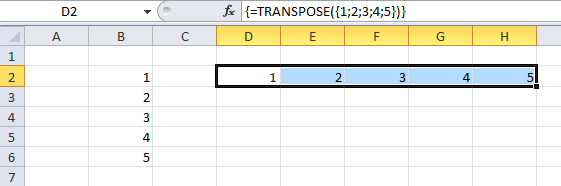
Array formula in cell D2:H2:

Range B2:B6 has 1 column and 5 rows and it is a vertical range. Use the TRANSPOSE function to convert it to a horizontal range. Shown in the example above.

When is the TRANSPOSE function useful?

The TRANSPOSE function is most useful in scenarios where you want to manipulate arrays which is often the case when using more complicated functions like MMULT function and other Excel functions that take arrays as an input value.

However, simple comparison test between two different arrays may require the TRANSPOSE function based on their layout on the worksheet. Here is an example:

The image above shows two arrays, array1 is in cells C2:F2, and array2 is in C3:G3. To be able to compare these horizontal arrays also with different sizes, we need to transpose one of the arrays to be able to perform the comparison without errors.

Formula in cell C7:

Here is a quick break down:

1. TRANSPOSE(C3:G3): The formula in cell C7 transposes array2 in cells C3:G3 from horizontal to vertical.
2. C2:F2=TRANSPOSE(C3:G3): The equal sign compares the values despite being in different sizes.

The image above shows the comparisons in cells C7:F11, the grey values above and to the left of C7:F11 show the arrays: array1 and array2

2. Syntax

TRANSPOSE(array)

=TRANSPOSE(B2:B6) is entered in cell range D2:H2, as an array formula.

3. How to enter an array formula

1. Select cell range D2:H2.
2. Press with left mouse button on in the formula bar.
3. Type: =TRANSPOSE(B2:B6) in the formula bar.
4. Press and hold CTRL + SHIFT simultaneously.
5. Press Enter once.
6. Release CTRL + SHIFT.

If you did this right the formula now begins and ends with a curly bracket. Like this: {=TRANSPOSE(B2:B6)} Don't enter these characters yourself.

Back to top

3.1 Why do I have to enter the TRANSPOSE function as an array formula?

It returns more than one value, you need to enter it as an array formula if you want to see all values on the worksheet.

Back to top

3.2 Excel 365 users can enter the TRANSPOSE function as a regular formula

Excel 365 users can now enter dynamic array formulas as regular formulas. Dynamic array formulas expand automatically, this is called spilling.

Back to top

4. What happens if you transpose a range with the same number of columns and rows?

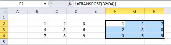
The picture shows what happens if you transpose a cell range with the same number of rows and columns, in this case, a cell range with 3 columns and 3 rows.

The range size doesn't change but the numbers in the range change positions. The values in the first column (B2:B4) is converted into the first row (F2:H2), the same with the second column (C2:C4) into the second row (F3:H3), and so on.

Back to top

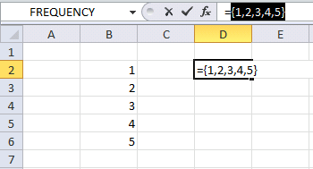
5. How to converting a vertical cell range to constants

This animated picture shows how to convert the values in a cell range to constants.

What the animated picture doesn't show you is that I am pressing F9 after selecting the cell range B2:B6. These are all the steps:

1. Select cell D2.
2. Type =
3. Select cell range B2:B6.
4. Press F9.

The formula bar returns {1;2;3;4;5}. The curly brackets tell you that it is an array. The constants in the array are separated by semicolons. The semicolon tells you that the next value is in the row below. In the example above all values are separated vertically, this is a one-dimensional array.

Back to top

6. Transpose a vertical array with constants

What happens if we transpose this array? {1;2;3;4;5}  Select a cell and type in formula bar: =TRANSPOSE({1;2;3;4;5}) Press F9.

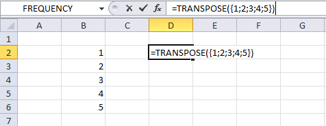
The formula bar shows {1,2,3,4,5}. The comma tells you that the values in the array are separated horizontally.

You can verify this by selecting D2:H2, type =TRANSPOSE({1;2;3;4;5}) in the formula bar and enter it as an array formula.

In other words, the colon tells you that the next value in the array is in the next column. The semicolon tells you that the next value is in the row below.

Back to top

7. Two-dimensional arrays

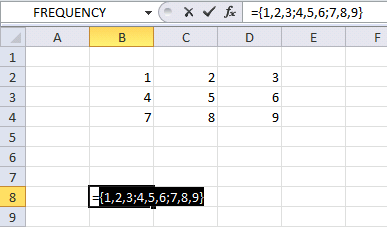
Look at this array {1,2,3;4,5,6;7,8,9}. You can now distinguish that this array has 3 columns and 3 rows by looking at the commas and semicolons. The array has values in more than one column and one row. This is a two-dimensional array.

I made this array {1,2,3;4,5,6;7,8,9} from cell range B2:D4, it has 3 columns and 3 rows.

Back to top

8. Transpose a cell range manually without using a formula

1. Select a cell range you want to transpose
2. Copy cells (CTRL + c)
3. Press with right mouse button on on a destination cell
4. Press with left mouse button on "Paste Special..."
   
5. Press with left mouse button on "Transpose"
6. Press with left mouse button on OK button

Back to top

9. Function not working

The TRANSPOSE function

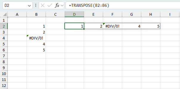
• propagates error values if present in the source data.
• returns a #NAME! error if you misspell the function name.

9.1 Troubleshooting the error value

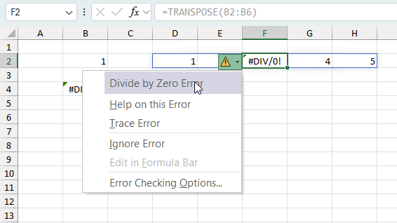
When you encounter an error value in a cell a warning symbol appears, displayed in the image above. Press with mouse on it to see a pop-up menu that lets you get more information about the error.

1. The first line describes the error if you press with left mouse button on it.
2. The second line opens a pane that explains the error in greater detail.
3. The third line takes you to the "Evaluate Formula" tool, a dialog box appears allowing you to examine the formula in greater detail.
4. This line lets you ignore the error value meaning the warning icon disappears, however, the error is still in the cell.
5. The fifth line lets you edit the formula in the Formula bar.
6. The sixth line opens the Excel settings so you can adjust the Error Checking Options.

Here are a few of the most common Excel errors you may encounter.

#NULL error - This error occurs most often if you by mistake use a space character in a formula where it shouldn't be. Excel interprets a space character as an intersection operator. If the ranges don't intersect an #NULL error is returned. The #NULL! error occurs when a formula attempts to calculate the intersection of two ranges that do not actually intersect. This can happen when the wrong range operator is used in the formula, or when the intersection operator (represented by a space character) is used between two ranges that do not overlap. To fix this error double check that the ranges referenced in the formula that use the intersection operator actually have cells in common.

#SPILL error - The #SPILL! error occurs only in version Excel 365 and is caused by a dynamic array being to large, meaning there are cells below and/or to the right that are not empty. This prevents the dynamic array formula expanding into new empty cells.

#DIV/0 error - This error happens if you try to divide a number by 0 (zero) or a value that equates to zero which is not possible mathematically.

#VALUE error - The #VALUE error occurs when a formula has a value that is of the wrong data type. Such as text where a number is expected or when dates are evaluated as text.

#REF error - The #REF error happens when a cell reference is invalid. This can happen if a cell is deleted that is referenced by a formula.

#NAME error - The #NAME error happens if you misspelled a function or a named range.

#NUM error - The #NUM error shows up when you try to use invalid numeric values in formulas, like square root of a negative number.

#N/A error - The #N/A error happens when a value is not available for a formula or found in a given cell range, for example in the VLOOKUP or MATCH functions.

#GETTING_DATA error - The #GETTING_DATA error shows while external sources are loading, this can indicate a delay in fetching the data or that the external source is unavailable right now.

7.2 The formula returns an unexpected value

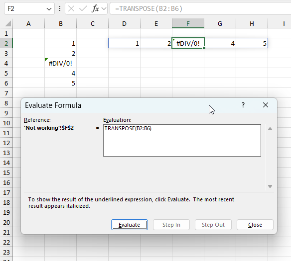
To understand why a formula returns an unexpected value we need to examine the calculations steps in detail. Luckily, Excel has a tool that is really handy in these situations. Here is how to troubleshoot a formula:

1. Select the cell containing the formula you want to examine in detail.
2. Go to tab “Formulas” on the ribbon.
3. Press with left mouse button on "Evaluate Formula" button. A dialog box appears.
   The formula appears in a white field inside the dialog box. Underlined expressions are calculations being processed in the next step. The italicized expression is the most recent result. The buttons at the bottom of the dialog box allows you to evaluate the formula in smaller calculations which you control.
4. Press with left mouse button on the "Evaluate" button located at the bottom of the dialog box to process the underlined expression.
5. Repeat pressing the "Evaluate" button until you have seen all calculations step by step. This allows you to examine the formula in greater detail and hopefully find the culprit.
6. Press "Close" button to dismiss the dialog box.

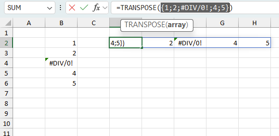
There is also another way to debug formulas using the function key F9. F9 is especially useful if you have a feeling that a specific part of the formula is the issue, this makes it faster than the "Evaluate Formula" tool since you don't need to go through all calculations to find the issue..

1. Enter Edit mode: Double-press with left mouse button on the cell or press F2 to enter Edit mode for the formula.
2. Select part of the formula: Highlight the specific part of the formula you want to evaluate. You can select and evaluate any part of the formula that could work as a standalone formula.
3. Press F9: This will calculate and display the result of just that selected portion.
4. Evaluate step-by-step: You can select and evaluate different parts of the formula to see intermediate results.
5. Check for errors: This allows you to pinpoint which part of a complex formula may be causing an error.

The image above shows cell reference B2:B6 converted to hard-coded value using the F9 key. The TRANSPOSE function works with non-error values which is not the case in this example. We have found what is wrong with the formula.

Tips!

• View actual values: Selecting a cell reference and pressing F9 will show the actual values in those cells.
• Exit safely: Press Esc to exit Edit mode without changing the formula. Don't press Enter, as that would replace the formula part with the calculated value.
• Full recalculation: Pressing F9 outside of Edit mode will recalculate all formulas in the workbook.

Remember to be careful not to accidentally overwrite parts of your formula when using F9. Always exit with Esc rather than Enter to preserve the original formula. However, if you make a mistake overwriting the formula it is not the end of the world. You can “undo” the action by pressing keyboard shortcut keys CTRL + z or pressing the “Undo” button

7.3 Other errors

Floating-point arithmetic may give inaccurate results in Excel - Article

Floating-point errors are usually very small, often beyond the 15th decimal place, and in most cases don't affect calculations significantly.

Get the Excel file

How-to-use-the-TRANSPOSE-function.xlsx

Useful links

TRANSPOSE function - Microsoft

'TRANSPOSE' function examples

5 easy ways to extract Unique Distinct Values
First, let me explain the difference between unique values and unique distinct values, it is important you know the difference […]

5 easy ways to VLOOKUP and return multiple values
This post explains how to lookup a value and return multiple values. No array formula required.

A beginners guide to Excel array formulas
Array formulas allows you to do advanced calculations not possible with regular formulas.

Functions in 'Lookup and reference' category

The TRANSPOSE function function is one of 25 functions in the 'Lookup and reference' category.

Excel categories

Leave a Comment