Extract a list of duplicates from a column
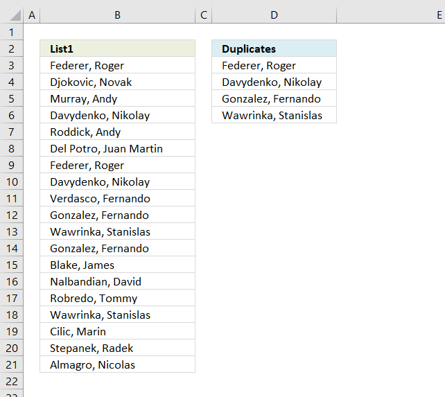
The array formula in cell C2 extracts duplicate values from column A. Only one duplicate of each value is displayed in column C.
The following link takes you to an article that shows formulas that extract duplicates from a source range spread out to multiple columns: Extract duplicates from a multi-column cell range
What's on this page
- Extract duplicates - older Excel versions
- Extract duplicates - Excel 365
- Filter duplicates - Excel Table
- Filter duplicates - Autofilter
- Filter duplicates - User Defined Function
- List duplicates based on condition
- Filter duplicate values and sort by corresponding date
- Extract a list of duplicates from two columns combined
- Filter duplicate words from a cell range - UDF
- List duplicate rows / records
- Extract a list of alphabetically sorted duplicates from a column
- Filter duplicates within same date, week or month
- Label groups of duplicate records
- Extract a list of alphabetically sorted duplicates based on a condition
- Extract a list of alphabetically sorted duplicates based on a condition - Excel 365
- Extract duplicate values without exceptions
- Extract duplicate values without exceptions - Excel 365
- Get *.xlsx file
- Extract a list of duplicates from three columns combined - Excel 365
- Extract a list of duplicates from three columns combined - earlier Excel versions
1. Extract duplicates
Update 2017-08-19! New regular formula in cell D3:
This video explains how to use the formula and how it works
The following formula is an outdated formula, the above formula is smaller and better.
Array formula in D3:
1.1 How to enter an array formula
- Copy (Ctrl + c) above formula
- Double press with left mouse button on cell C2
- Paste (Ctrl + v) to cell C2
- Press and hold CTRL + SHIFT simultaneously
- Press Enter once
- Release all keys
Your formula now looks like this: {=array_formula}
Don't enter the curly brackets, they appear automatically.
Recommended articles

Array formulas allows you to do advanced calculations not possible with regular formulas.
1.2 How to copy the formula
Copy cell C2 and paste it to cells below as far as needed.
1.3 Remove #num errors:
Copy cell C2 and paste it down to D20.
Learn more:
Recommended articles
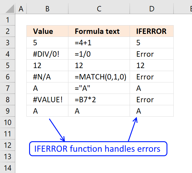
The IFERROR function lets you catch most errors in Excel formulas. It was introduced in Excel 2007. In previous Excel […]
1.4 Earlier Excel versions, array formula in C2:
The IFERROR function was introduced in Excel 2007, if you have an earlier version then use the formula above.
How (the old) array formula works
Step 1 - Display a duplicate value only once
COUNTIF(D2:$D$2, $B$3:$B$21) contains both a relative and absolute reference (D2:$D$2) to a range.
returns the array
{0; 0; 0; ... ; 0}
When you copy a cell reference like this the cell reference expands.
Recommended articles

Counts the number of cells that meet a specific condition.
Step 2 - Filter values in $A$2:$A$20 having duplicates
The COUNTIF function counts the number of cells within a range that meet the given condition.
COUNTIF($B$3:$B$21, $B$3:$B$21)
returns
{2; 1; 1; ... ; 1}.
COUNTIF($B$3:$B$21, $B$3:$B$21)>1
returns
{TRUE; FALSE; FALSE; ... ; FALSE}
IF(COUNTIF($B$3:$B$21, $B$3:$B$21)>1, 0, 1)
returns {1; 0; 0;... ; 0}
Step 3 - Calculate arrays combined
COUNTIF(D2:$D$2, $B$3:$B$21)+IF(COUNTIF($B$3:$B$21, $B$3:$B$21)>1, 0, 1)
{0; 0; 0; ... ; 0} + {1; 0; 0; ... ; 0}
equals {1; 0; 0; ... ; 0}
Step 4 - Identify duplicates
MATCH(0, COUNTIF(D2:$D$2, $B$3:$B$21)+IF(COUNTIF($B$3:$B$21, $B$3:$B$21)>1, 0, 1), 0)
returns 2.
Match returns the relative position of an item in an array that matches a specified value.
Recommended articles
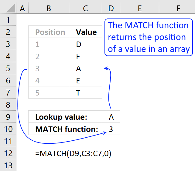
Identify the position of a value in an array.
Step 5 - Return duplicates
INDEX function returns a value or reference of the cell at the intersection of a particular row and column, in a given range
INDEX($B$3:$B$21, MATCH(0, COUNTIF(D2:$D$2, $B$3:$B$21)+IF(COUNTIF($B$3:$B$21, $B$3:$B$21)>1, 0, 1), 0))
becomes
INDEX($B$3:$B$21, 2)
and returns "Federer, Roger".
Recommended articles
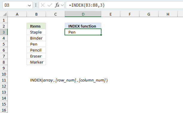
Gets a value in a specific cell range based on a row and column number.
Final thoughts
When the formula in c2 is copied to c3 the reference changes.
Example
The formula in c2: =INDEX($A$2:$A$20, MATCH(0, COUNTIF(D2:$D$2, $A$2:$A$20)+IF(COUNTIF($A$2:$A$20, $A$2:$A$20)>1, 0, 1), 0))
Then copy the formula to C3.
The formula references changes: =INDEX($A$2:$A$20, MATCH(0, COUNTIF(D3:$D$2, $A$2:$A$20)+IF(COUNTIF($A$2:$A$20, $A$2:$A$20)>1, 0, 1), 0))
Read more about absolute and relative cell references.
This makes it possible to avoid previous cell values (C2) and only calculate the remaining values.
2. Extract duplicates - Excel 365

The image above shows a list of values in column B, some of them are duplicates. The formula in cell D3 extracts duplicate values in cell D3 and cells below.
Excel 365 dynamic array formula in cell D3:
The formula extracts only one duplicate per value, remove the UNIQUE function from the formula above to list all instances of each duplicate. The formula spills values to cell D3 and cells below automatically, a #SPILL error indicates that one or more cells below cell C3 are non-empty. Remove the values so the formula can display all duplicates.
2.1 Explaining formula
Step 1 - Count values
The COUNTIF function counts cells based on a condition or criteria, this allows us to identify duplicate values.
COUNTIF(range, criteria)
returns {2; 1; 1; ... ; 1}.
Step 2 - Identify duplicates
The larger than sign lets you check if a number is larger than 1, in other words, a duplicate.
COUNTIF(B3:B21, B3:B21)>1
returns {TRUE; FALSE; FALSE; ... ; FALSE}.
Step 3 - Filter values if count is larger than 1
The FILTER function extracts values/rows based on a condition or criteria.
FILTER(array, include, [if_empty])
FILTER(B3:B21, COUNTIF(B3:B21, B3:B21)>1)
returns {"Federer, Roger "; "Davydenko, Nikolay "; ... ; "Wawrinka, Stanislas "}.
Step 4 - List one instance of each value
The UNIQUE function extracts both unique and unique distinct values and also compare columns to columns or rows to rows.
UNIQUE(array,[by_col],[exactly_once])
UNIQUE(FILTER(B3:B21, COUNTIF(B3:B21, B3:B21)>1))
returns {"Federer, Roger "; "Davydenko, Nikolay "; "Gonzalez, Fernando "; "Wawrinka, Stanislas "}.
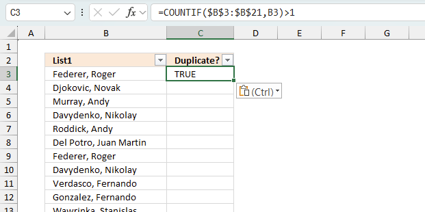
3. Filter duplicates - Excel Table
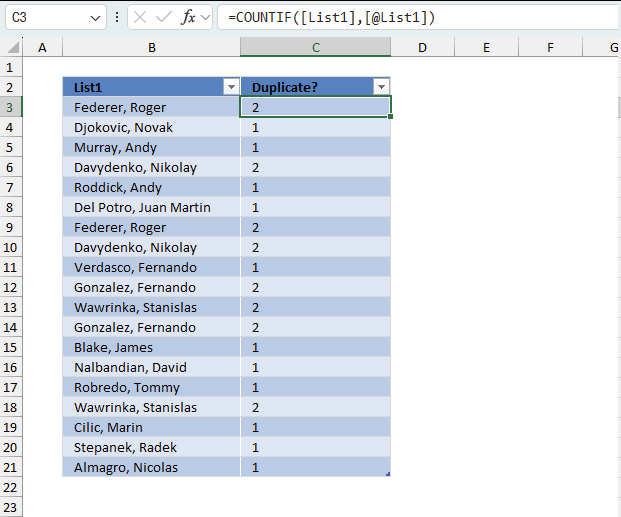
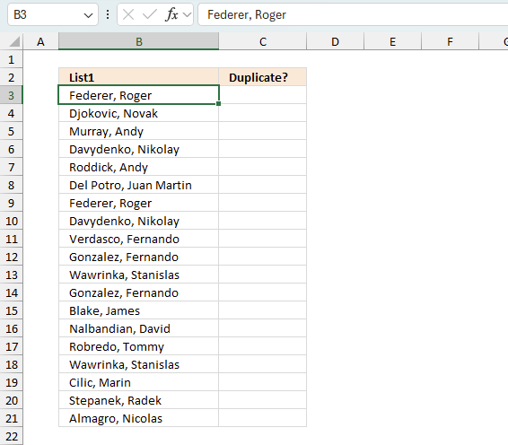
The image above shows an Excel Table in cells B2:C21, it contains names in column B and some of the names are repeated meaning there are duplicates. Column C is a "helper" column since Excel Tables don't have a built-in feature to list only duplicates. The "helper" column in cells C2:C21 has the following formula:
Enter this formula in the first cell in column C which is C3. The formula is automatically entered to the remaining cells without any user interaction. This is a feature of Excel Tables. The cell references used in Excel Tables are called structured references and work differently compared to regular cell references.
- [List1] - This refers to the entire column named "List1" in your table. The square brackets without @ indicate you want to reference all values in that column.
- [@List1] - This refers to the current row's value in the "List1" column. The @ symbol means "this row."
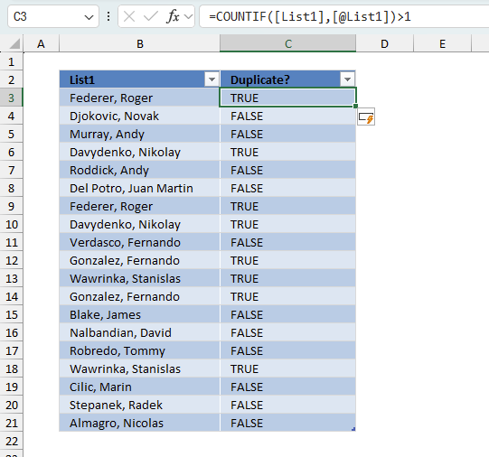
The formula counts the number of instances of each value in column Benchmark, for example, cell B3 contains "Federer, Roger" and the formula on the corresponding cell in column C displays 2 meaning there is another instance of "Federer, Roger" somewhere in the list. This means that a number larger than 1 indicates that there is at least one duplicate. We can now change the formula using the larger than signs:
The larger than sign is a logical operator meaning the expression will return a boolean value TRUE or FALSE. It returns TRUE if the number is larger than one and FALSE if the number is equal to 1.
We can use boolean values to filter the Excel Table. Next to the header names are a button containing a down-pointing arrow or triangle.
- Press with left mouse button on that button to the right of header name "Duplicate?". A popup menu appears.
- Make sure that only boolean value TRUE is selected. See the image above.
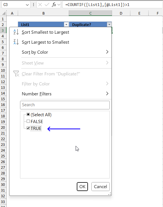
- Press with left mouse button on the OK button to apply the changes.
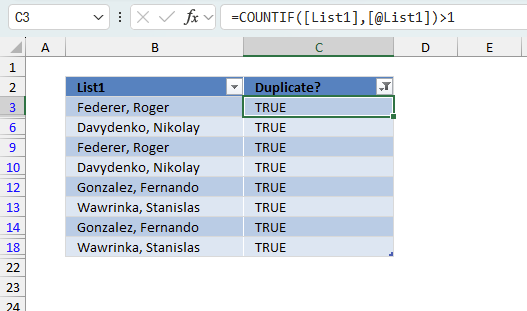
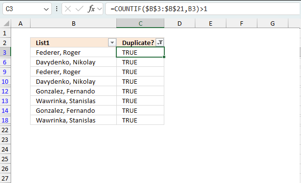
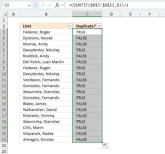
The image above shows the filtered Excel Table. You can see that all row numbers are not shown in the row column and the visible ones are blue. This means that some of the rows are hidden or "filtered out". Being more specific, only boolean values TRUE in column C are visible. Note! This method shows all duplicates in contrast to one instance of each duplicate.
4. Filter duplicates using Autofilter
This example demonstrates how to filter duplicates using Autofilter. The image above shows values in column B, the Autofilter applied to column C filters duplicates. The table shows blue row numbers meaning the data set is filtered.
4.1 How to apply Autofilter
- Select a populated cell in the data set.
- Go to tab "Data" on the ribbon.
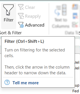
- Press with left mouse button on the "Filter button" on the ribbon or press shortcut keys Ctrl + Shift + L) to turn on filtering for the selected cells.
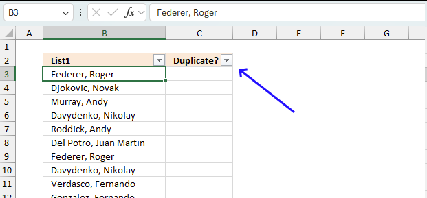
Buttons containing arrows appear next to the column header names.
4.2 Duplicate formula
You need a formula to filter duplicates as the autofilter feature can't filter duplicates on it's own. Enter the following regular formula in cell C3:
=COUNTIF($B$3:$B$21,B3)>1
Make sure to use absolute cell references in the first argument, this allows the formula to "lock" this cell reference meaning it won't change when we copy the cell and paste to cells below. The COUNTIF function allows you to count each instance and it has at least one duplicate if the count is larger than 1. The larger than sign checks if the output from the COUNTIF function is larger than 1. It returns TRUE if the expression is true and FALSE if the expression is 1.
Now copy cell C3 and paste to cells below as far as needed.
4.3 Apply filter
- Press with left mouse button on the arrow button next to column hear name "Duplicate?"
- A popup menu appears.
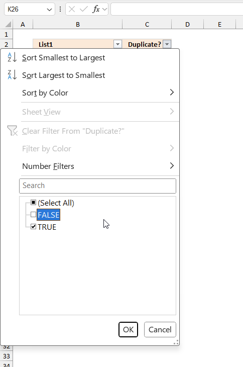
- Deselect "FALSE" by disable the check box next to "False".
- Press with left mouse button on the "OK" button to apply the filter.
4.4 Clear the filter
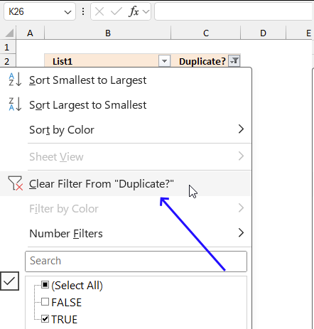
To clear the filter simply press the arrow button again and press with left mouse button on "Clear Filter From Duplicate?" displayed on the popup menu that appears. Then press the "OK" button.
5. Filter duplicates in a large dataset - UDF

This article demonstrates a user defined function that extracts duplicate values and also count duplicates.
Example, the image below shows a list containing duplicate values.

User defined function
Function DuplicateValues(rng As Variant, Optional CountDuplicates As Variant) As Variant

Dim Test As New Collection

Dim Dupes As New Collection

Dim Value As Variant

Dim Item As Variant

Dim temp() As Variant

ReDim temp(0)

rng = rng.Value

If IsMissing(CountDuplicates) Then CountDuplicates = False

On Error Resume Next

For Each Value In rng

If Len(Value) > 0 Then Test.Add Value, CStr(Value)

If Err Then

If Len(Value) > 0 Then Dupes.Add Value, CStr(Value)

Err = False

End If

Next Value

On Error GoTo 0

If CountDuplicates = False Then

For Each Item In Dupes

temp(UBound(temp)) = Item

ReDim Preserve temp(UBound(temp) + 1)

Next Item

DuplicateValues = Application.Transpose(temp)

Else

DuplicateValues = Dupes.Count

End If

End Function
How to add the user defined function to your workbook
- Press Alt-F11 to open the Visual Basic editor
- Press with left mouse button on Module on the Insert menu
- Copy and paste the above user defined function
- Exit visual basic editor
How to extract duplicate values
- Select a cell range
- Type =DuplicateValues($A$1:$F$3000, FALSE)
- Press and hold CTRL + SHIFT simultaneously
- Press Enter once
- Release all keys
How to count duplicate values
- Select a cell
- Type =DuplicateValues($A$1:$F$3000, TRUE) into formula bar and press ENTER.
6. List duplicates based on condition
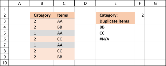
Question: How do I filter duplicates based on a condition?
Answer: Column B contains category and column C contains Items. Only duplicate Items with adjacent Category number 2 is listed in column E.
AA is in category 2 (row 3) and 1 but exists only once in category 2. It is not a duplicate.
BB is in category 2 and exists twice (row 4 and 9). BB has a duplicate.
CC is in category 2 and has a duplicate (row 6 and 8). CC is a duplicate.
Excel 365 dynamic array formula in cell E4:
Formula for earlier Excel versions in cell E4:
6.1 Explaining formula in cell E4
Step 1 - Identify values that has not been displayed before
COUNTIF($E$3:E3, $C$3:$C$9)=0
returns {TRUE;TRUE;TRUE;... ;TRUE}
In cell E4 no values has been shown before so the array returns TRUE for all values.
Recommended articles
Counts the number of cells that meet a specific condition.
Step 2 - Find duplicates in category 2
COUNTIFS($B$3:$B$9, $F$2, $C$3:$C$9, $C$3:$C$9)>1
returns {FALSE;TRUE; FALSE;TRUE;FALSE; TRUE;TRUE}
Recommended articles
Checks multiple conditions against the same number of cell ranges and counts how many times all criteria are met.
Step 3 - Multiply arrays
(COUNTIF($E$3:E3, $C$3:$C$9)=0)*(COUNTIFS($B$3:$B$9, $F$2, $C$3:$C$9, $C$3:$C$9)>1)
returns {0;1; 0;1;0; 1;1}
Step 4 - Divide 1 with array
1/(((COUNTIF($E$3:E3, $C$3:$C$9)=0)*(COUNTIFS($B$3:$B$9, $F$2, $C$3:$C$9, $C$3:$C$9)>1)))
returns {#DIV/0!; 1;#DIV/0!; 1;#DIV/0!; 1;1}
Step 5 - Find last matching value in array
The LOOKUP function ignores errors but requires the second argument to be sorted ascending. However our list contains only errors or 1 so the LOOKUP function returns the last matching 1 in the array.
LOOKUP(2, 1/(((COUNTIF($E$3:E3, $C$3:$C$9)=0)*(COUNTIFS($B$3:$B$9, $F$2, $C$3:$C$9, $C$3:$C$9)>1))), $C$3:$C$9)
returns "BB" in cell E4. BB is the corresponding value to the last 1 in the array, bolded above.
Recommended articles
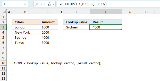
Finds a value in a sorted cell range and returns a value on the same row.
Step 6 - Relative cell refences
The following cell reference is both an absolute and relative cell reference: $E$3:E3. When you copy the formula to cells below, the cell ref changes. That way the formula knows which values have been displayed before.
Recommended articles
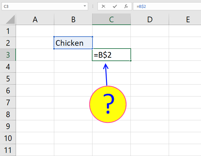
What is a reference in Excel? Excel has an A1 reference style meaning columns are named letters A to XFD […]
Get excel example file
Filter duplicates with a condition.xlsx
(Excel Workbook *.xlsx)
7. Filter duplicate values and sort by corresponding date

This section demonstrates formulas that extract duplicates from cell range B2:B21 and sort the output by the corresponding dates specified in cell range A2:A21.
Excel 365 dynamic array formula in cell D2:
The Excel 365 formula above spills values to cells below and to the right automatically. A #SPILL error indicates that one or more cells are not empty, make sure the cells are empty so the formula can show all values.
Array formula for earlier Excel versions in D2:
Array formula for earlier Excel versions in E2:
7.1 Explaining formula in cell D2
Step 1 - Identify duplicates
The COUNTIF function counts values based on a condition or criteria.
COUNTIF($B$2:$B$21, $B$2:$B$21)>1
returns {TRUE; TRUE; TRUE; ... ; TRUE}.
Step 2 - Convert boolean values
The IF function returns a value based on a logical expression, TRUE returns argument2 and FALSE returns argument3.
IF(COUNTIF($B$2:$B$21, $B$2:$B$21)>1, COUNTIF($A$2:$A$21, "<"&$A$2:$A$21), "")
The COUNTIF function returns a rank number indicating the position if the list were sorted, "<" is concatenated with A$2:$A$21 to make the COUNTIF function behave in this way.
returns {7;11;8; ... ;4}
Step 3 - Extract the k/th smallest number in array
The SMALL function returns the k/th smallest number in array ignoring blanks.
SMALL(IF(COUNTIF($B$2:$B$21,$B$2:$B$21)>1,COUNTIF($A$2:$A$21,"<"&$A$2:$A$21),""),ROWS($A$1:A1))
returns 0 (zero).
Step 4 - Identify position in cell range
The MATCH function returns the position of a value in a cell range or an array.
MATCH(SMALL(IF(COUNTIF($B$2:$B$21, $B$2:$B$21)>1, COUNTIF($A$2:$A$21, "<"&$A$2:$A$21), ""),ROWS($A$1:A1)), COUNTIF($A$2:$A$21, "<"&$A$2:$A$21), 0)
returns 10.
Step 5 - Return value from cell range
INDEX($A$2:$A$21, MATCH(SMALL(IF(COUNTIF($B$2:$B$21, $B$2:$B$21)>1, COUNTIF($A$2:$A$21, "<"&$A$2:$A$21), ""),ROWS($A$1:A1)), COUNTIF($A$2:$A$21, "<"&$A$2:$A$21), 0))
returns "1/10/2008" in cell D2.
Get Excel *.xlsx file
Filter duplicate values and sort by datev2.xlsx
8. Extract a list of duplicates from two columns combined
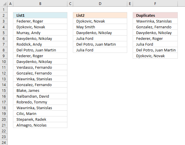
The following regular formula extracts duplicates from column B (List1) and column D (List2) combined, the result is shown in column F.
Formula in cell F3:
Excel 365 dynamic array formula in cell F3:
8.1 Explaining formula in cell F3
This formula consists of two similar parts, one returns values from List1 and the other returns values from List2.
IFERROR(formula1, formula2)
Step 1 - Prevent duplicate values
The COUNTIF function counts values based on a condition, in this case, I am counting values in cells above. This makes sure that duplicates are ignored.
COUNTIF($F$2:F2,$B$3:$B$21)=0
returns
{TRUE;TRUE;TRUE; ... ;TRUE}
Step 2 - Count values in List1
We want to know where the duplicates are if there are any.
COUNTIF($B$3:$B$21,$B$3:$B$21)>1
returns {TRUE;FALSE; FALSE;... ; FALSE}
Step 3 - Multiply arrays
(COUNTIF($F$2:F2,$B$3:$B$21)=0)*(COUNTIF($B$3:$B$21,$B$3:$B$21)>1)
returns {1;0;0;... ;0}
Step 4 - Divide 1 with array
The LOOKUP function ignores error and if we divide 1 with 0 an error occurs. 1/0 = #DIV/0!
1/((COUNTIF($F$2:F8,$B$3:$B$21)=0)*(COUNTIF($B$3:$B$21,$B$3:$B$21)>1))
returns {1;#DIV/0!;... ;#DIV/0!}
Step 5 - Return value based on array
LOOKUP(2, 1/((COUNTIF($F$2:F2,$B$3:$B$21)=0)*(COUNTIF($B$3:$B$21,$B$3:$B$21)>1)), $B$3:$B$21)
returns Wawrinka, Stanislas in cell F3.
Step 6 - Return values from List2
When values run out from List1 formula1 returns errors, the IFERROR function then moves to formula2.
IFERROR(formula1, formula2)
formula2 is just like formula1 except that it returns values from List2 and duplicates found between List1 and List2.
Earlier Excel versions:
Get Excel *.xlsx
how-to-extract-a-list of duplicates from two columns-in-excelv2.xlsx
9. Filter duplicate words from a cell range - UDF

AJ Serrano asks:
I have a column where each rows contains different values and I wanted to obtain the duplicate values in each rows.
SAMPLE
COLUMN A contains these data:
3M - Asia
3M South America
3M - Africa
3M - US
3M - ASIA
3M - Us
3M - South AMERICA
3M - Europe
3M Australia
3M Australia
3M Europe
3M aSIA
3M US
How do I get duplicate values and put them on the next column say column B? 3M is one of the duplicate values.
Answer:
Rick Rothstein (MVP - Excel) helped me out here with a powerful user defined function (udf).
Array formula in cell B2:B9
Select all the cells to be filled, then type the above formula into the Formula Bar and press CTRL+SHIFT+ENTER
Array formula in cell C2:C9
Select all the cells to be filled, then type the above formula into the Formula Bar and press CTRL+SHIFT+ENTER
User defined function

Instructions
- You can select far more cells to load the formulas in than are required by the list. The empty text string will be displayed for cells not having an entry.
- You can specify a larger range than the there are filled in cells as the argument to these macros to allow for future entries in the column.
- You can specify whether the listing is to be case sensitive or not via the optional second argument with the default value being FALSE, meaning duplicated entries with different casing like One, one, ONE, onE, etc.. will all be treated as if they were the same word with the same spelling. If you pass TRUE for that optional second argument, then those words would all be treated as if they were different words.
- For all the "Case Insensitive" listing, the words are listed in Proper Case (first letter upper case, remaining letters lower case). The reason being if you had One, one and ONE then there is not reason to prefer one version over another, so I solved the problem by using Proper Case throughout.
VBA Code:
Function DuplicatedWords(Rng As Range, Optional CaseSensitive As Boolean) As Variant
  Dim X As Long, WordCount As Long, List As String, Duplicates As Variant, Words() As String
  List = WorksheetFunction.Trim(Replace(Join(WorksheetFunction.Transpose(Rng)), Chr(160), " "))
  Words = Split(List)
  For X = 0 To UBound(Words)
    If CaseSensitive Then
      If UBound(Split("  " & List & "  ", " " & Words(X) & " ")) > 1 Then
        Duplicates = Duplicates & Words(X) & " "
        List = Replace(List, Words(X), "", 1, -1, vbBinaryCompare)
      End If
    Else
      If UBound(Split(" " & UCase(List) & " ", " " & UCase(Words(X)) & " ")) > 1 Then
        Duplicates = Duplicates & StrConv(Words(X), vbProperCase) & " "
        List = Replace(List, Words(X), "", 1, -1, vbTextCompare)
      End If
    End If
  Next
  Duplicates = WorksheetFunction.Trim(Duplicates)
  Words = Split(Duplicates)
  If Application.Caller.Count > UBound(Words) Then
    Duplicates = Duplicates & Space(Application.Caller.Count - UBound(Words))
  End If
  DuplicatedWords = WorksheetFunction.Transpose(Split(Duplicates))
End Function
How to implement user defined function in excel
- Press Alt-F11 to open visual basic editor
- Press with left mouse button on Module on the Insert menu
- Type your user defined function
- Exit visual basic editor
- Select a sheet
- Select a cell range
- Type =DuplicatedWords($A$2:$A$18, TRUE) into formula bar and press CTRL+SHIFT+ENTER
Get Rick Rothstein's Excel example file
Many thanks to Rick Rothstein (Mvp - Excel)!!
10. List duplicate rows / records
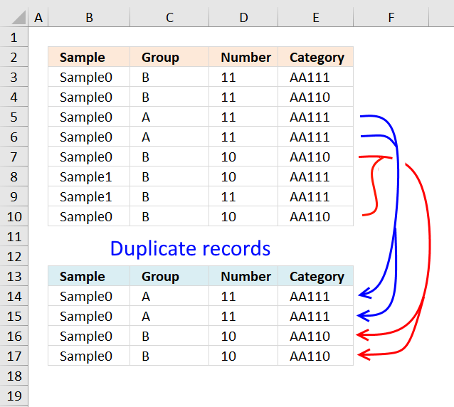
This article describes how to filter duplicate rows with the use of a formula. It is, in fact, an array formula which is demonstrated below. The function that makes this all possible is the COUNTIFS function, introduced in Excel 2007.
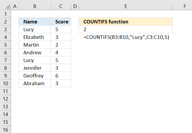
The COUNTIFS function evaluates criteria to cells across multiple ranges and counts the number of times all criteria are met.
Array formula in cell A30:
Copy cell A30 and paste it to the right as far as needed. Then copy cells and paste them down as far as needed.
Excel 365 dynamic array formula in cell B14:
How this formula works in cell A30
Step 1 - Find duplicates
COUNTIFS($A$2:$A$25, $A$2:$A$25, $B$2:$B$25, $B$2:$B$25, $C$2:$C$25, $C$2:$C$25, $D$2:$D$25, $D$2:$D$25)>1
returns this array: {False, False, True, ... , True}
Step 2 - Use array to extract row numbers
IF({False, False, True, ... , True}, ROW($A$2:$A$25)-MIN(ROW($A$2:$A$25))+1)
returns this array:
{False, False, 3, ... , 24}
Step 3 - Return the k-th smallest value
SMALL(IF(COUNTIFS($A$2:$A$25, $A$2:$A$25, $B$2:$B$25, $B$2:$B$25, $C$2:$C$25, $C$2:$C$25, $D$2:$D$25, $D$2:$D$25)>1, ROW($A$2:$A$25)-MIN(ROW($A$2:$A$25))+1), ROW(A1))
returns 3.
Step 4 - Return a value of the cell at the intersection of a particular row and column
INDEX($A$2:$D$25, SMALL(IF(COUNTIFS($A$2:$A$25, $A$2:$A$25, $B$2:$B$25, $B$2:$B$25, $C$2:$C$25, $C$2:$C$25, $D$2:$D$25, $D$2:$D$25)>1, ROW($A$2:$A$25)-MIN(ROW($A$2:$A$25))+1), ROW(A1)), COLUMN(A1))
returns "Sample1"
Final notes
The formula uses relative and absolute cell references.
In cell B30 the array formula changes cell references to:
=INDEX($A$2:$D$25, SMALL(IF(COUNTIFS($A$2:$A$25, $A$2:$A$25, $B$2:$B$25, $B$2:$B$25, $C$2:$C$25, $C$2:$C$25, $D$2:$D$25, $D$2:$D$25)>1, ROW($A$2:$A$25)-MIN(ROW($A$2:$A$25))+1), ROW(A1)), COLUMN(B1))
In cell A31 the formula changes cell references to:
=INDEX($A$2:$D$25, SMALL(IF(COUNTIFS($A$2:$A$25, $A$2:$A$25, $B$2:$B$25, $B$2:$B$25, $C$2:$C$25, $C$2:$C$25, $D$2:$D$25, $D$2:$D$25)>1, ROW($A$2:$A$25)-MIN(ROW($A$2:$A$25))+1), ROW(A2)), COLUMN(A2))
Get excel sample file for this tutorial.
Filter-duplicate-rows-in-excel-2007v3.xlsx
(Excel 2007 Workbook *.xlsx)
11. Extract a list of alphabetically sorted duplicates from a column
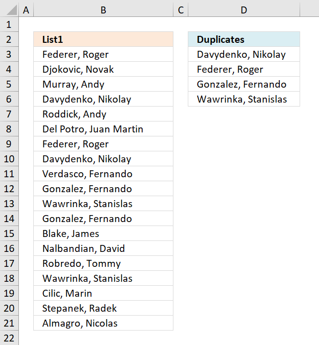
The following formulas extracts duplicate values sorted from A to Z from cell range B3:B21.
Excel 365 dynamic array formula in cell C2:
The formula above extracts all duplicates and sorts them alphabetically. However, if you want only one instance of each duplicate then use this formula:
The following formula is for older Excel versions, array formula in C2:
How to enter an array formula
Skip these steps if you are an Excel 365 subscriber. Excel 365 lets you enter all kinds of formulas as regular formulas.
- Copy above formula
- Double press with left mouse button on cell D3
- Paste formula to cell D3
- Press and hold CTRL + SHIFT simultaneously
- Press Enter once
- Release all keys
The formula now looks like this: {=arrayformula}
Don't enter the curly brackets yourself, they appear automatically.
11.1 Explaining formula in cell C2
Step 1 - Count values
The COUNTIF fucntion counts values based on a condition or criteria, this way we can identify which values are duplicates and which are not.
COUNTIF($B$3:$B$21,$B$3:$B$21)
returns {2;1;1;... ;1}.
Step 2 - Display first instance of each duplicate
The following COUNTIF function makes sure that the output list only contains unique values. The first argument contains a cell reference that expands as the formula is copied to cells below.
COUNTIF(D2:$D$2,$B$3:$B$21)<>1
returns {TRUE; TRUE; TRUE; ... ; TRUE}.
Step 3 - Multiply arrays
Both values must return TRUE.
COUNTIF($B$3:$B$21,$B$3:$B$21)*(COUNTIF(D2:$D$2,$B$3:$B$21)
returns {2; 1; 1; ... ; 1}.
| Boolean | Boolean | Multiply |
| FALSE | FALSE | 0 |
| FALSE | TRUE | 0 |
| TRUE | TRUE | 1 |
Step 4 - Replace TRUE with a number representing the order if list were sorted
The IF function returns a value based on a logical expression, if TRUE the second argument is returned, if FALSE the third argument.
IF(COUNTIF($B$3:$B$21,$B$3:$B$21)*(COUNTIF(D2:$D$2,$B$3:$B$21)<>1)>1,COUNTIF($B$3:$B$21,"<"&$B$3:$B$21),"")
returns {7;"";"";... ;""}.
Step 5 - Get smallest value in array
The MIN function returns the samllest value in a cell range or array.
MIN(IF(COUNTIF($A$2:$A$20, $A$2:$A$20)*IF(COUNTIF(C1:$C$1, $A$2:$A$20)=1, 0, 1)>1, COUNTIF($A$2:$A$20, "<"&$A$2:$A$20), ""))
returns 3.
Step 6 - Replace TRUE in array with a number representing the order if list were sorted
IF(COUNTIF($B$3:$B$21,$B$3:$B$21)>1,COUNTIF($B$3:$B$21,"<"&$B$3:$B$21),"")
returns {7;"";"";... ;""}.
Step 7 - Return relative position
MATCH(MIN(IF(COUNTIF($B$3:$B$21,$B$3:$B$21)*(COUNTIF(D2:$D$2,$B$3:$B$21)<>1)>1,COUNTIF($B$3:$B$21,"<"&$B$3:$B$21),"")),IF(COUNTIF($B$3:$B$21,$B$3:$B$21)>1,COUNTIF($B$3:$B$21,"<"&$B$3:$B$21),""),0)
returns 4.
Step 8 - Return value
The INDEX function returns a value from a cell range based on a row and column number. The cell range is a single column so the column number is not necessary.
INDEX($A$2:$A$20, MATCH(MIN(IF(COUNTIF($A$2:$A$20, $A$2:$A$20)*IF(COUNTIF(C1:$C$1, $A$2:$A$20)=1, 0, 1)>1, COUNTIF($A$2:$A$20, "<"&$A$2:$A$20), "")), IF(COUNTIF($A$2:$A$20, $A$2:$A$20)>1, COUNTIF($A$2:$A$20, "<"&$A$2:$A$20), ""), 0))
returns "Davydenko, Nikolay " in cell D3.
Get Excel *.xlsx file
how-to-extract-a-list-of-duplicates-sorted-a-to-z-from-a-columnv2.xlsx
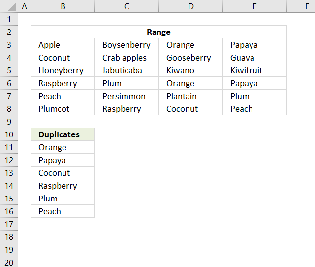
12. Filter duplicates within same date, week or month
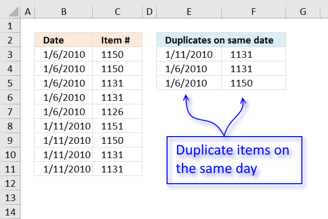
The image above demonstrates a formula in cell E3 that extracts duplicate items if they are on the same date.
Formula in E3:
Copy cell and paste it to cell range E3:F5.
10.1 Explaining formula in cell E3
Step 1 - Keep track of previous values
The COUNTIFS function calculates the number of cells across multiple ranges that equals all given conditions. If a date and corresponding item already has been displayed the function returns 1. The cell references grow when the cell is copied to cells below, the formula keeps track of previously shown values.
COUNTIFS($E$2:$E2, $B$3:$B$11, $F$2:$F2, $C$3:$C$11)=0
returns {TRUE; TRUE;... ; TRUE}
Step 2 - Find duplicates
COUNTIFS($B$3:$B$11, $B$3:$B$11, $C$3:$C$11, $C$3:$C$11)>1
becomes {2;2;2;2;1;1;1;2;2}>1
and returns {TRUE; TRUE; ... ; TRUE}
Step 3 - Multiply arrays
We use AND logic because both conditions must be met.
(COUNTIFS($E$2:$E2, $B$3:$B$11, $F$2:$F2, $C$3:$C$11)=0)*(COUNTIFS($B$3:$B$11, $B$3:$B$11, $C$3:$C$11, $C$3:$C$11)>1)
returns {1;1;1;1;0;0;0;1;1}
Step 4 - Divide 1 with array
The LOOKUP function ignores error values and this is what we are going to use. In order to get an error if a value in the array is FALSE or 0 (zero) we divide 1 with 0 and excel returns !DIV/0 error.
1/((COUNTIFS($E$2:$E2, $B$3:$B$11, $F$2:$F2, $C$3:$C$11)=0)*(COUNTIFS($B$3:$B$11, $B$3:$B$11, $C$3:$C$11, $C$3:$C$11)>1))
becomes 1/{1;1;1;1;0;0;0;1;1} and returns {1;1;1;1;#DIV/0!;#DIV/0!;#DIV/0!;1;1}
Step 5 - Get value
The LOOKUP function returns a value on the corresponding row if it is not an error value, simplified.
LOOKUP(2, 1/((COUNTIFS($E$2:$E2, $B$3:$B$11, $F$2:$F2, $C$3:$C$11)=0)*(COUNTIFS($B$3:$B$11, $B$3:$B$11, $C$3:$C$11, $C$3:$C$11)>1)), B$3:B$11)
returns 40189 (1/11/2010) in cell E3.
Get Excel *.xlsx file
Filter-duplicates-within-same-date-week-month-year.xlsx
12.2 Filter duplicates within same week

Formula in B16:
Array formula in F16:
Copy cell and paste it down as far as needed.
Array formula in G16:
Copy cell and paste it down as far as needed.
12.3 Filter duplicates within same month

Array formula in F29:
Copy cell and paste it down as far as needed.
Array formula in G29:
Copy cell and paste it down as far as needed.
Get the Excel File here
Filter-duplicates-within-same-date-week-month-year.xls
(Excel 97-2003 Workbook *.xls)
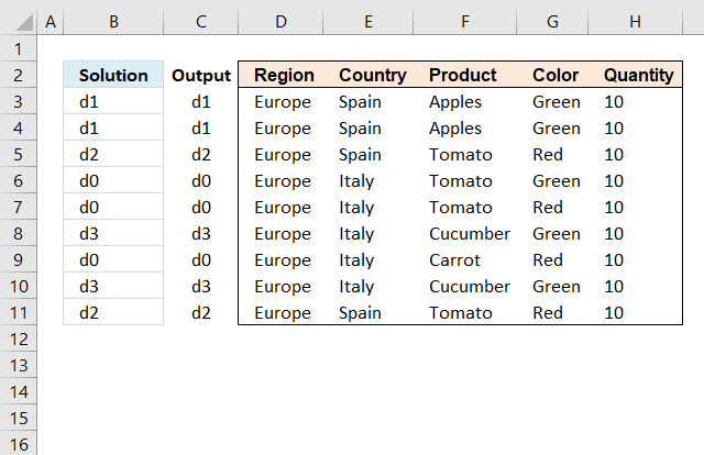
13. Label groups of duplicate records
Michael asks:
I need to identify the duplicates based on the Columns D:H and put in Column C a small “d” + a running number for the duplicates which are duplicated the same.
If no duplicates only to put in a “d0” for instance.

Answer
The following array formula assigns unique records the label "d0" and duplicate records the same label
Array formula in cell B3:
To enter an array formula, type the formula in a cell then press and hold CTRL + SHIFT simultaneously, now press Enter once. Release all keys.
The formula bar now shows the formula with a beginning and ending curly bracket telling you that you entered the formula successfully. Don't enter the curly brackets yourself.
How to copy array formula
- Select cell B3.
- Copy cell (Ctrl + c).
- Select cell range B4:B11.
- Paste to cell range (Ctrl + v).
Explaining formula in cell B3

Step 1 - Identify if record is unique
The COUNTIFS function allows you to count cells based on multiple conditions.
COUNTIFS($D$3:$D$11, D3, $E$3:$E$11, E3, F$3:$F$11, F3, $G$3:$G$11, G3, $H$3:$H$11, H3)=1
becomes
COUNTIFS({"Europe"; "Europe"; "Europe"; "Europe"; "Europe"; "Europe"; "Europe"; "Europe"; "Europe"},"Europe",{"Spain"; "Spain"; "Spain"; "Italy"; "Italy"; "Italy"; "Italy"; "Italy"; "Spain"},"Spain",{"Apples"; "Apples"; "Tomato"; "Tomato"; "Tomato"; "Cucumber"; "Carrot"; "Cucumber"; "Tomato"},"Apples",{"Green"; "Green"; "Red"; "Green"; "Red"; "Green"; "Red"; "Green"; "Red"},"Green",{10; 10; 10; 10; 10; 10; 10; 10; 10},10)=1
becomes
2=1
and returns the boolean value FALSE. It means that the record is not unique, in other words, there is at least one other duplicate record.
Step 2 - Return "d0" if record is unique
The IF function has three arguments, the first one must be a logical expression. If the expression evaluates to TRUE then one thing happens (argument 2) and if FALSE another thing happens (argument 3).
The previous step returns TRUE or FALSE an we are going to use that in our IF function.
IF(COUNTIFS($D$3:$D$11, D3, $E$3:$E$11, E3, F$3:$F$11, F3, $G$3:$G$11, G3, $H$3:$H$11, H3)=1, "d0", remaining_formula)
becomes
IF(FALSE, "d0", remaining_formula)
and the calculation continues in the last IF argument.
Step 3 - Is record the first of all duplicate records?
COUNTIFS($D$3:D3, D3, $E$3:E3, E3, $F$3:F3, F3, $G$3:G3, G3)=1
becomes
1=1
and returns TRUE.
Step 4 - Calculate number if record is first record
IF(COUNTIFS($D$3:D3, D3, $E$3:E3, E3, $F$3:F3, F3, $G$3:G3, G3)=1, "d"&(SUM(1/COUNTIFS($D$3:D3, $D$3:D3, $E$3:E3, $E$3:E3, F$3:F3, $F$3:F3, $G$3:G3, $G$3:G3, $H$3:H3, $H$3:H3))-SUM(IF(COUNTIFS($D$3:$D$11, $D$3:D3, $E$3:$E$11, $E$3:E3, F$3:$F$11, $F$3:F3, $G$3:$G$11, $G$3:G3, $H$3:$H$11, $H$3:H3)=1, 1, 0))), remaining_formula)
becomes
IF(TRUE, "d"&(SUM(1/COUNTIFS($D$3:D3, $D$3:D3, $E$3:E3, $E$3:E3, F$3:F3, $F$3:F3, $G$3:G3, $G$3:G3, $H$3:H3, $H$3:H3))-SUM(IF(COUNTIFS($D$3:$D$11, $D$3:D3, $E$3:$E$11, $E$3:E3, F$3:$F$11, $F$3:F3, $G$3:$G$11, $G$3:G3, $H$3:$H$11, $H$3:H3)=1, 1, 0))), remaining_formula)
becomes
IF(TRUE, "d"&(SUM(1/1)-SUM(IF(COUNTIFS($D$3:$D$11, $D$3:D3, $E$3:$E$11, $E$3:E3, F$3:$F$11, $F$3:F3, $G$3:$G$11, $G$3:G3, $H$3:$H$11, $H$3:H3)=1, 1, 0))), remaining_formula)
becomes
IF(TRUE, "d"&(SUM(1/1)-SUM(IF(2=1, 1, 0))), remaining_formula)
becomes
IF(TRUE, "d"&(SUM(1/1)-SUM(IF(FALSE, 1, 0))), remaining_formula)
becomes
IF(TRUE, "d"&(1-0), remaining_formula)
becomes
IF(TRUE, "d"&1, remaining_formula)
and returns "d1" in cell B3.
Step 5 - Get value from the first duplicate record
This part of the formula is rund if the record is NOT the first duplicate of a specific record in the list, it finds the first record and returns that value.
In cell B4 the formula changes to the following line because of absolute and relative cell references.
INDEX($B$3:B4, MIN(IF(COUNTIFS(D4, $D$3:D4, E4, $E$3:E4, F4, $F$3:F4, G4, $G$3:G4, H4, $H$3:H4), MATCH(ROW($D$3:D4), ROW($D$3:D4)), ""))))
becomes
INDEX($B$3:B4, MIN(IF({1;1}, MATCH(ROW($D$3:D4), ROW($D$3:D4)), ""))))
becomes
INDEX($B$3:B4, MIN(IF({1;1}, {1; 2}, ""))))
becomes
INDEX($B$3:B4, MIN({1; 2}))
becomes
INDEX($B$3:B4, 1)
becomes
INDEX({"d1";"d1"}, 1)
and returns "d1" in cell B4.
The INDEX function returns a value based on a cell reference and column/row numbers.
14. Extract a list of alphabetically sorted duplicates based on a condition

Array formula in cell E5:
14.1 How to enter an array formula
- Copy (Ctrl + c) above formula
- Double press with left mouse button on cell E5
- Paste formula to cell E5
- Press and hold CTRL + SHIFT simultaneously
- Press Enter once
- Release all keys
The formula now looks like this: {=arrayformula}
Don't enter the curly brackets yourself, they appear automatically.
14.2 Explaining formula in cell E5
You can easily follow along, select cell E5. Go to tab "Formulas" on the ribbon and press with left mouse button on the "Evaluate Formula" button.
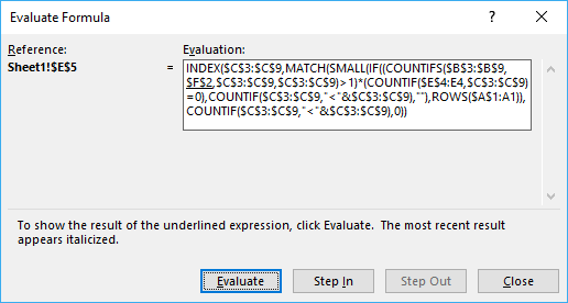
Then press with left mouse button on "Evaluate" button to move to next step.
Step 1 - Check if category matches condition
COUNTIFS($B$3:$B$9, $F$2, $C$3:$C$9, $C$3:$C$9)>1
becomes
COUNTIFS($B$3:$B$9, $F$2, $C$3:$C$9, $C$3:$C$9)>1
becomes
COUNTIFS({"Winter"; "Winter"; "Winter"; "Summer"; "Winter"; "Summer"; "Winter"},"Winter",{"Skates"; "Ski"; "Skates"; "Fishing rod"; "Sledge"; "Fishing rod"; "Sledge"},{"Skates"; "Ski"; "Skates"; "Fishing rod"; "Sledge"; "Fishing rod"; "Sledge"})>1
and returns
{2;1;2;0;2;0;2}
Step 2 - Check if count is larger than 1
This allows us to filter duplicate values.
COUNTIFS($B$3:$B$9, $F$2, $C$3:$C$9, $C$3:$C$9)>1
becomes
{2;1;2;0;2;0;2}>1
and returns {TRUE; FALSE; TRUE; FALSE; TRUE; FALSE; TRUE}
Step 3 - Count previous values in list
COUNTIF($E$4:E4, $C$3:$C$9)
returns {0;0;0;0;0;0;0}
Step 4 - Check if they have not been shown before
This makes sure that previous values in column E are not repeated.
COUNTIF($E$4:E4, $C$3:$C$9)>0
becomes
{0;0;0;0;0;0;0}=0
and returns {TRUE; TRUE; TRUE; TRUE; TRUE; TRUE; TRUE}
Step 5 - Multiply arrays
(COUNTIFS($B$3:$B$9, $F$2, $C$3:$C$9, $C$3:$C$9)>1)*(COUNTIF($E$4:E4, $C$3:$C$9)=0)
becomes
{TRUE; FALSE; TRUE; FALSE; TRUE; FALSE; TRUE}*{TRUE; TRUE; TRUE; TRUE; TRUE; TRUE; TRUE}
and returns {1;0;1;0;1;0;1}
Step 6 - Build an array of sort ranking numbers
COUNTIF($C$3:$C$9, "<"&$C$3:$C$9) returns {2;4;2;0;5;0;5}
Step 7 - Return corresponding sort rank number
IF((COUNTIFS($B$3:$B$9, $F$2, $C$3:$C$9, $C$3:$C$9)>1)*(COUNTIF($E$4:E4, $C$3:$C$9)=0), COUNTIF($C$3:$C$9, "<"&$C$3:$C$9), "")
becomes
IF({1;0;1;0;1;0;1},{2;4;2;0;5;0;5}, "")
and returns {2;"";2;"";5;"";5}
Step 8 - Find the n-th smallest number
SMALL(IF((COUNTIFS($B$3:$B$9, $F$2, $C$3:$C$9, $C$3:$C$9)>1)*(COUNTIF($E$4:E4, $C$3:$C$9)=0), COUNTIF($C$3:$C$9, "<"&$C$3:$C$9), ""), ROWS($A$1:A1))
becomes
SMALL({2;"";2;"";5;"";5}, ROWS($A$1:A1))
becomes
SMALL({2;"";2;"";5;"";5}, 1)
and returns 2.
Step 9 - Get the positions of values in the array
MATCH(SMALL(IF((COUNTIFS($B$3:$B$9, $F$2, $C$3:$C$9, $C$3:$C$9)>1)*(COUNTIF($E$4:E4, $C$3:$C$9)=0), COUNTIF($C$3:$C$9, "<"&$C$3:$C$9), ""), ROWS($A$1:A1)), COUNTIF($C$3:$C$9, "<"&$C$3:$C$9), 0)
becomes
MATCH(2, COUNTIF($C$3:$C$9, "<"&$C$3:$C$9), 0)
becomes
MATCH(2, {2;4;2;0;5;0;5}, 0)
and returns 1.
Step 10 - Return value in data set based on coordinate
INDEX($C$3:$C$9, MATCH(SMALL(IF((COUNTIFS($B$3:$B$9, $F$2, $C$3:$C$9, $C$3:$C$9)>1)*(COUNTIF($E$4:E4, $C$3:$C$9)=0), COUNTIF($C$3:$C$9, "<"&$C$3:$C$9), ""), ROWS($A$1:A1)), COUNTIF($C$3:$C$9, "<"&$C$3:$C$9), 0))
becomes
INDEX($C$3:$C$9, 1)
becomes
INDEX({"Skates";"Ski";"Skates";"Fishing rod";"Sledge";"Fishing rod";"Sledge"}, 5)
and returns "Skates" in cell E5.
15. Extract a list of alphabetically sorted duplicates based on a condition - Excel 365

Formula in cell F5:
13.1 Explaining formula in cell F5
Step 1 - Check condition
The equal sign checks if the condition is equal to values in cell range B3:B9.
B3:B9=F2
becomes
{"Winter";"Winter";"Winter";"Summer";"Winter";"Summer";"Winter"}="Winter"
and returns
{TRUE; TRUE; TRUE; FALSE; TRUE; FALSE; TRUE}
Step 2 - Filter values based on criteria
The FILTER function filters values in a given cell range based on a condition or criteria.
FILTER(C3:C9, B3:B9=F2)
becomes
FILTER({"Skates"; "Ski"; "Skates"; "Fishing rod"; "Sledge"; "Fishing rod"; "Sledge"}, {TRUE; TRUE; TRUE; FALSE; TRUE; FALSE; TRUE})
and returns
{"Skates"; "Ski"; "Skates"; "Sledge"; "Sledge"}.
Step 3 - Assign a formula to a name
The LET function lets you assign a formula to a name. This reduces the formula size significantly.
FILTER(C3:C9, (B3:B9=F2) is assigned to z.
LET(z, FILTER(C3:C9, (B3:B9=F2)), formula)
Step 3 - Match filtered values
The MATCH function returns a number representing the relative position of an item in an array or cell range.
MATCH(z, z, 0)
becomes
MATCH({"Skates";"Ski";"Skates";"Sledge";"Sledge"}, {"Skates";"Ski";"Skates";"Sledge";"Sledge"}, 0)
and returns {1; 2; 1; 4; 4}.
Step 4 - Create a sequence based on the number of filtered values
The SEQUENCE function returns a sequence of numbers.
SEQUENCE(rows, [columns], [start], [step])
SEQUENCE(ROWS(z))
becomes
SEQUENCE(5)
and returns {1; 2; 3; 4; 5}.
Step 5 - Check for duplicates
The less than and greater than characters return TRUE if the numbers don't match indicating that the value is a duplicate.
MATCH(z, z, 0)<>SEQUENCE(ROWS(z))
becomes
{1; 2; 1; 4; 4}={1; 2; 3; 4; 5}
and returns {TRUE; TRUE; FALSE; TRUE; FALSE}.
Step 6 - Filter values
FILTER(z, MATCH(z, z, 0)<>SEQUENCE(ROWS(z)))
becomes
FILTER({"Skates"; "Ski"; "Skates"; "Sledge"; "Sledge"}, {TRUE; TRUE; FALSE; TRUE; FALSE})
and returns {"Skates";"Sledge"}.
Step 6 - Sort array
The SORT function sorts values in a cell range or array from A to Z.
SORT(FILTER(z, MATCH(z, z, 0)<>SEQUENCE(ROWS(z))))
becomes
SORT({"Skates";"Sledge"})
and returns {"Skates";"Sledge"}.
16. Extract duplicate values with exceptions

This example demonstrates a formula for earlier versions, Excel 2019, and previous versions. I recommend the smaller formula demonstrated in section 2 if you use Excel 365.
Array formula in cell F3:
16.1 How to enter an array formula
- Copy above array formula.
- Double press on cell F3.
- Paste formula to cell F3 (CTRL + v).
- Press and hold CTRL + SHIFT simultaneously.
- Press Enter once.
- Release all keys.
The formula now begins with and ends with a curly bracket, this is Excel letting you know the formula is an array formula.
Don't enter these characters yourself, they appear automatically.
16.2 Explaining the formula in cell F2
Step 1 - Count values
The COUNTIF function calculates the number of cells that is equal to a condition.
Function syntax: COUNTIF(range, criteria)
COUNTIF($B$3:$B$21, $B$3:$B$21)
becomes
COUNTIF({"Federer, Roger ";"Djokovic, Novak "; ... ;"Almagro, Nicolas "},{"Federer, Roger ";"Djokovic, Novak "; ... ;"Almagro, Nicolas "})
and returns
{2; 1; 1; 2; 1; 1; 2; 2; 1; 2; 2; 2; 1; 1; 1; 2; 1; 1; 1}
Step 2 - Check if the count number is larger than 1
The larger than sign is a logical operator, it returns TRUE or FALSE.
COUNTIF($B$3:$B$21, $B$3:$B$21)>1
becomes
{2; 1; 1; 2; 1; 1; 2; 2; 1; 2; 2; 2; 1; 1; 1; 2; 1; 1; 1}>1
and returns
{TRUE; FALSE; FALSE; ... ; FALSE}.
Step 3 - Check if previous results are not in $B$3:$B$21
$F$2:F2 is a cell reference to the cell above F3, it grows when the cell is copied to cells below. This makes it possible to keep track of previous results.
COUNTIF($F$2:F2, $B$3:$B$21)=0
becomes
COUNTIF("Duplicates",{"Federer, Roger ";"Djokovic, Novak ";"Murray, Andy "; ... ;"Almagro, Nicolas "})=0
becomes
{0; 0; 0; 0; 0; 0; 0; 0; 0; 0; 0; 0; 0; 0; 0; 0; 0; 0; 0}=0
and returns
{TRUE; TRUE; TRUE; ... ; TRUE}
Step 4 - Count excluded values in $B$3:$B$21
COUNTIF($D$3:$D$4, $B$3:$B$21)<>1
becomes
COUNTIF({"Federer, Roger ";"Gonzalez, Fernando "},{"Federer, Roger ";"Djokovic, Novak ";"Murray, Andy "; ... ;"Almagro, Nicolas "})<>1
becomes
{1; 0; 0; 0; 0; 0; 1; 0; 0; 1; 0; 1; 1; 0; 0; 0; 0; 0; 0}<>1
and returns
{FALSE;TRUE;TRUE; ... ;TRUE}
Step 5 - Multiply arrays - AND logic
The asterisk character lets you multiply numbers and boolean values in an Excel formula.
AND logic means that both conditions must be met, in other words, both arrays must contain TRUE in order to return TRUE.
TRUE * TRUE = TRUE (1)
TRUE * FALSE = FALSE (0)
FALSE * TRUE = FALSE (0)
FALSE * FALSE = FALSE (0)
When you multiply boolean values TRUE or FALSE the result is their numerical equivalent:
TRUE = 1
FALSE = 0 (zero)
(COUNTIF($B$3:$B$21, $B$3:$B$21)>1)*(COUNTIF($F$2:F2, $B$3:$B$21)=0)*(COUNTIF($D$3:$D$4, $B$3:$B$21)<>1)
becomes
{TRUE; FALSE; FALSE; ... ; FALSE}* {TRUE; TRUE; TRUE; ... ; TRUE} * {FALSE;TRUE;TRUE; ... ;TRUE}
and returns
{0; 0; 0; 1; 0; 0; 0; 1; 0; 0; 1; 0; 0; 0; 0; 1; 0; 0; 0}
Step 6 - Divide 1 by the array
The division character lets you divide numbers and boolean values in an Excel formula. Some numbers in the array above are 0 (zero) and some are 1. You can't divide a number by 0 (zero), Excel returns an error value.
However, the LOOKUP function ignores errors which we can take advantage of in this formula.
1/((COUNTIF($B$3:$B$21, $B$3:$B$21)>1)*(COUNTIF($F$2:F2, $B$3:$B$21)=0)*(COUNTIF($D$3:$D$4, $B$3:$B$21)<>1))
becomes
1/{0; 0; 0; 1; 0; 0; 0; 1; 0; 0; 1; 0; 0; 0; 0; 1; 0; 0; 0}
and returns
{#DIV/0!; #DIV/0!; #DIV/0!; 1; ... ; #DIV/0!}.
Step 7 - Return value
The LOOKUP function find a value in a cell range and return a corresponding value on the same row.
Function syntax: LOOKUP(lookup_value, lookup_vector, [result_vector])
LOOKUP(2, 1/((COUNTIF($B$3:$B$21, $B$3:$B$21)>1)*(COUNTIF($F$2:F2, $B$3:$B$21)=0)*(COUNTIF($D$3:$D$4, $B$3:$B$21)<>1)), $B$3:$B$21)
becomes
LOOKUP(2, {#DIV/0!; #DIV/0!; #DIV/0!; 1; ... ; #DIV/0!}, {"Federer, Roger ";"Djokovic, Novak "; ... ;"Almagro, Nicolas "},{"Federer, Roger ";"Djokovic, Novak "; ... ;"Almagro, Nicolas "})
and returns
"Wawrinka, Stanislas ".
Step 8 - Replace error values
The IFERROR function if the value argument returns an error, the value_if_error argument is used. If the value argument does NOT return an error, the IFERROR function returns the value argument.
Function syntax: IFERROR(value, value_if_error)
The formula returns error values when it runs out of values, the IFERROR function displays nothing when that happens.
IFERROR(LOOKUP(2, 1/((COUNTIF($B$3:$B$21, $B$3:$B$21)>1)*(COUNTIF($F$2:F2, $B$3:$B$21)=0)*(COUNTIF($D$3:$D$4, $B$3:$B$21)<>1)), $B$3:$B$21), "")
17. Extract duplicate values with exceptions - Excel 365

The following formula is a dynamic array formula and is entered as a regular formula, it works only in Excel 365.
Formula in cell F3:
17.1 Explaining array formula in cell F2
Step 1 - Check if the value is a duplicate
The COUNTIF function counts values based on a condition. It can also be used to count multiple values.
COUNTIF(B3:B21, B3:B21)>1
becomes
COUNTIF({"Federer, Roger ";"Djokovic, Novak ";"Murray, Andy "; ... ;"Almagro, Nicolas "},{"Federer, Roger ";"Djokovic, Novak ";"Murray, Andy "; ... ;"Almagro, Nicolas "})>1
becomes
{3; 1; 1; 2; 1; 1; 3; 2; 1; 2; 2; 2; 3; 1; 1; 2; 1; 1; 1}>1
The larger than character checks if the numbers in the array is larger than 1. The output is TRUE or FALSE.
{3; 1; 1; 2; 1; 1; 3; 2; 1; 2; 2; 2; 3; 1; 1; 2; 1; 1; 1}>1
returns
{TRUE; FALSE; FALSE; ... ; FALSE}.
Step 2 - Check if the value is in the exceptions list
This step returns an array that shows if the values are in the exceptions list or not.
COUNTIF(D3:D4, B3:B21)=0
becomes
COUNTIF({"Federer, Roger ";"Gonzalez, Fernando "},{"Federer, Roger ";"Djokovic, Novak ";"Murray, Andy "; ... ;"Almagro, Nicolas "})=0
and returns
{FALSE; TRUE; TRUE; ... ; TRUE}.
Step 3 - Apply AND logic
The asterisk lets you multiply the arrays. It returns TRUE only if both arrays contain TRUE.
TRUE * TRUE = TRUE (1)
FALSE* TRUE = FALSE (0)
TRUE * FALSE= FALSE (0)
FALSE * FALSE= FALSE (0)
Note that the boolean values are converted into their numerical equivalents, TRUE = 1, and FALSE = 0 (zero).
(COUNTIF(B3:B21,B3:B21)>1)*(COUNTIF(D3:D4,B3:B21)=0)
becomes
{TRUE; FALSE; FALSE; ... ; FALSE} * {FALSE; TRUE; TRUE; ... ; TRUE}
and returns
{0; 0; 0; 1; 0; 0; 0; 1; 0; 0; 1; 0; 0; 0; 0; 1; 0; 0; 0}
Step 4 - Filter values
The FILTER function extracts values/rows based on a condition or criteria.
Function syntax: FILTER(array, include, [if_empty])
FILTER(B3:B21,(COUNTIF(B3:B21,B3:B21)>1)*(COUNTIF(D3:D4,B3:B21)=0))
becomes
FILTER(B3:B21, {0; 0; 0; 1; 0; 0; 0; 1; 0; 0; 1; 0; 0; 0; 0; 1; 0; 0; 0})
becomes
FILTER({"Federer, Roger "; "Djokovic, Novak "; "Murray, Andy "; ... ; "Almagro, Nicolas "}, {0; 0; 0; 1; 0; 0; 0; 1; 0; 0; 1; 0; 0; 0; 0; 1; 0; 0; 0})
and returns
{"Davydenko, Nikolay "; "Davydenko, Nikolay "; "Wawrinka, Stanislas "; "Wawrinka, Stanislas "}.
Step 5 - Extract unique distinct values
The UNIQUE function returns a unique or unique distinct list.
Function syntax: UNIQUE(array,[by_col],[exactly_once])
UNIQUE(FILTER(B3:B21,(COUNTIF(B3:B21,B3:B21)>1)*(COUNTIF(D3:D4,B3:B21)=0)))
becomes
UNIQUE({"Davydenko, Nikolay "; "Davydenko, Nikolay "; "Wawrinka, Stanislas "; "Wawrinka, Stanislas "})
and returns
{"Davydenko, Nikolay "; "Wawrinka, Stanislas "}.
Step 6 - Shorten the formula
The LET function lets you name intermediate calculation results which can shorten formulas considerably and improve performance.
Function syntax: LET(name1, name_value1, calculation_or_name2, [name_value2, calculation_or_name3...])
UNIQUE(FILTER(B3:B21,(COUNTIF(B3:B21,B3:B21)>1)*(COUNTIF(D3:D4,B3:B21)=0)))
x - B3:B21
LET(x,B3:B21,UNIQUE(FILTER(x,(COUNTIF(x,x)>1)*(COUNTIF(D3:D4,x)=0))))
18. Get Excel *.xlsx file
19. Extract a list of duplicates from two or more columns combined - Excel 365
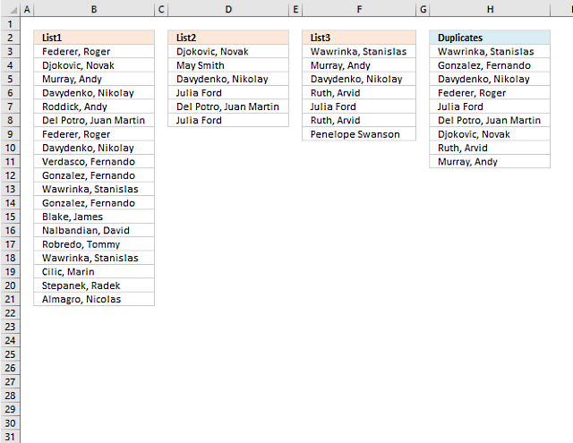
This example demonstrates how to list duplicates from three cell ranges combined, the first cell range is B3:B21, the second cell range is D3:D8 and the third is F3:F9.
Note, the cell ranges are not adjacent and are in different sizes. The result is an array shown in cell H3 and cells below as far as needed. This is called spilling in Excel 365.
Excel 365 dynamic array formula in cell H3:
You are not limited to three cell ranges, you can use up to 254 cell ranges.
19.1 Explaining the formula in cell H3
Step 1 - Combine cell ranges
The TOCOL function rearranges values in 2D cell ranges to a single column.
Function syntax: TOCOL(array, [ignore], [scan_by_col])
The TOCOL function lets you combine multiple cell ranges by adding parentheses and commas as delimiting characters.
TOCOL((B3:B21,D3:D8,F3:F9))
returns
{"Federer, Roger "; "Djokovic, Novak "; "Murray, Andy "; "Davydenko, Nikolay "; "Roddick, Andy "; "Del Potro, Juan Martin "; "Federer, Roger "; "Davydenko, Nikolay "; "Verdasco, Fernando "; "Gonzalez, Fernando "; "Wawrinka, Stanislas "; "Gonzalez, Fernando "; "Blake, James "; "Nalbandian, David "; "Robredo, Tommy "; "Wawrinka, Stanislas "; "Cilic, Marin "; "Stepanek, Radek "; "Almagro, Nicolas "; "Djokovic, Novak "; "May Smith"; "Davydenko, Nikolay "; "Julia Ford"; "Del Potro, Juan Martin "; "Julia Ford"; "Wawrinka, Stanislas "; "Murray, Andy "; "Davydenko, Nikolay "; "Ruth, Arvid"; "Julia Ford"; "Ruth, Arvid"; "Penelope Swanson"}.
Step 2 - Match values to the same values
The MATCH function returns the relative position of an item in an array that matches a specified value in a specific order.
Function syntax: MATCH(lookup_value, lookup_array, [match_type])
MATCH(TOCOL((B3:B21,D3:D8,F3:F9)),TOCOL((B3:B21,D3:D8,F3:F9)),0)
becomes
MATCH({"Federer, Roger "; "Djokovic, Novak "; ... ; "Penelope Swanson"}, {"Federer, Roger "; "Djokovic, Novak "; ... ; "Penelope Swanson"}, 0)
and returns
{1; 2; 3; 4; 5; 6; 1; 4; 9; 10; 11; 10; 13; 14; 15; 11; 17; 18; 19; 2; 21; 4; 23; 6; 23; 11; 3; 4; 29; 23; 29; 32}.
Step 3 - Count rows in the array
The ROWS function calculate the number of rows in a cell range.
Function syntax: ROWS(array)
ROWS(TOCOL((B3:B21,D3:D8,F3:F9)))
becomes
ROWS({"Federer, Roger "; "Djokovic, Novak "; ... ; "Penelope Swanson"})
and returns
32. There are 32 rows (values) in the array.
Step 4 - Create a sequence from 1 to n
The SEQUENCE function creates a list of sequential numbers.
Function syntax: SEQUENCE(rows, [columns], [start], [step])
SEQUENCE(ROWS(TOCOL((B3:B21,D3:D8,F3:F9))))
becomes
SEQUENCE(32)
and returns
{1; 2; 3; 4; 5; 6; 7; 8; 9; 10; 11; 12; 13; 14; 15; 16; 17; 18; 19; 20; 21; 22; 23; 24; 25; 26; 27; 28; 29; 30; 31; 32}.
Step 5 - Check if the numbers are not equal to the sequence
The less than and larger than sign combined lets you perform "not equal to" in an Excel formula. The result is a boolean value TRUE or FALSE, however, in this case, the result is an array containing boolean values.
MATCH(TOCOL((B3:B21,D3:D8,F3:F9)),TOCOL((B3:B21,D3:D8,F3:F9)),0)<>SEQUENCE(ROWS(TOCOL((B3:B21,D3:D8,F3:F9))))
becomes
{1; 2; 3; 4; 5; 6; 1; 4; 9; 10; 11; 10; 13; 14; 15; 11; 17; 18; 19; 2; 21; 4; 23; 6; 23; 11; 3; 4; 29; 23; 29; 32}<>{1; 2; 3; 4; 5; 6; 7; 8; 9; 10; 11; 12; 13; 14; 15; 16; 17; 18; 19; 20; 21; 22; 23; 24; 25; 26; 27; 28; 29; 30; 31; 32}
and returns
{FALSE; FALSE; FALSE; FALSE; FALSE; FALSE; TRUE; TRUE; FALSE; FALSE; FALSE; TRUE; FALSE; FALSE; FALSE; TRUE; FALSE; FALSE; FALSE; TRUE; FALSE; TRUE; FALSE; TRUE; TRUE; TRUE; TRUE; TRUE; FALSE; TRUE; TRUE; FALSE}.
This array lets you identify duplicate values, their positions correspond to the position in cell ranges B3:B21, D3:D8, and F3:F9.
Step 6 - Filter values based on the boolean array
The FILTER function extracts values/rows based on a condition or criteria.
Function syntax: FILTER(array, include, [if_empty])
FILTER(TOCOL((B3:B21,D3:D8,F3:F9)),MATCH(TOCOL((B3:B21,D3:D8,F3:F9)),TOCOL((B3:B21,D3:D8,F3:F9)),0)<>SEQUENCE(ROWS(TOCOL((B3:B21,D3:D8,F3:F9)))))
becomes
FILTER({"Federer, Roger "; "Djokovic, Novak "; ... ; "Penelope Swanson"},{FALSE; FALSE; FALSE; ... ; FALSE})
and returns
{"Federer, Roger "; "Davydenko, Nikolay "; "Gonzalez, Fernando "; "Wawrinka, Stanislas "; "Djokovic, Novak "; "Davydenko, Nikolay "; "Del Potro, Juan Martin "; "Julia Ford"; "Wawrinka, Stanislas "; "Murray, Andy "; "Davydenko, Nikolay "; "Julia Ford"; "Ruth, Arvid"}.
Step 7 - Extract unique distinct values
The UNIQUE function returns a unique or unique distinct list.
Function syntax: UNIQUE(array,[by_col],[exactly_once])
UNIQUE(FILTER(TOCOL((B3:B21,D3:D8,F3:F9)),MATCH(TOCOL((B3:B21,D3:D8,F3:F9)),TOCOL((B3:B21,D3:D8,F3:F9)),0)<>SEQUENCE(ROWS(TOCOL((B3:B21,D3:D8,F3:F9))))))
becomes
UNIQUE({"Federer, Roger "; "Davydenko, Nikolay "; "Gonzalez, Fernando "; "... ; "Ruth, Arvid"})
and returns
{"Federer, Roger "; "Davydenko, Nikolay "; "Gonzalez, Fernando "; "Wawrinka, Stanislas "; "Djokovic, Novak "; "Del Potro, Juan Martin "; "Julia Ford"; "Murray, Andy "; "Ruth, Arvid"}
Step 8 - Shorten the formula
The LET function lets you name intermediate calculation results which can shorten formulas considerably and improve performance.
Function syntax: LET(name1, name_value1, calculation_or_name2, [name_value2, calculation_or_name3...])
UNIQUE(FILTER(TOCOL((B3:B21,D3:D8,F3:F9)),MATCH(TOCOL((B3:B21,D3:D8,F3:F9)),TOCOL((B3:B21,D3:D8,F3:F9)),0)<>SEQUENCE(ROWS(TOCOL((B3:B21,D3:D8,F3:F9))))))
x - TOCOL((B3:B21,D3:D8,F3:F9))
LET(x,TOCOL((B3:B21,D3:D8,F3:F9)),UNIQUE(FILTER(x,MATCH(x,x,0)<>SEQUENCE(ROWS(x)))))
20. Extract a list of duplicates from three columns combined
The following regular formula extracts duplicate values from column B (List1), D (List2) and F (List3) combined, the result is displayed in cell H3 and cells below.
Formula in cell H3:
20.1 Explaining formula in cell F3
This formula consists of three similar parts, one returns values from List1 and the second returns values from List2 and the third returns duplicates from List3.
IFERROR(IFERROR(formula1, formula2), formula3)
Step 1 - Prevent duplicate values in output
The COUNTIF function counts values based on a condition, in this case, I am counting values in cells above. This makes sure that duplicates are not returned.
COUNTIF($H$2:H2,$B$3:$B$21)=0
becomes
COUNTIF("Duplicates",$B$3:$B$21)=0
becomes
COUNTIF("Duplicates",{"Federer, Roger ";"Djokovic, Novak ";"Murray, Andy ";"Davydenko, Nikolay ";"Roddick, Andy ";"Del Potro, Juan Martin ";"Federer, Roger ";"Davydenko, Nikolay ";"Verdasco, Fernando ";"Gonzalez, Fernando ";"Wawrinka, Stanislas ";"Gonzalez, Fernando ";"Blake, James ";"Nalbandian, David ";"Robredo, Tommy ";"Wawrinka, Stanislas ";"Cilic, Marin ";"Stepanek, Radek ";"Almagro, Nicolas "})=0
{0;0;0;0;0;0;0;0;0;0;0;0;0;0;0;0;0;0;0}=0
and returns
{TRUE;TRUE;TRUE; TRUE;TRUE;TRUE;TRUE; TRUE;TRUE;TRUE;TRUE; TRUE;TRUE;TRUE;TRUE; TRUE;TRUE;TRUE;TRUE}
Step 2 - Count values in List1
We want to know where the duplicates are in List1.
COUNTIF($B$3:$B$21,$B$3:$B$21)>1
becomes
COUNTIF({"Federer, Roger ";"Djokovic, Novak ";"Murray, Andy ";"Davydenko, Nikolay ";"Roddick, Andy ";"Del Potro, Juan Martin ";"Federer, Roger ";"Davydenko, Nikolay ";"Verdasco, Fernando ";"Gonzalez, Fernando ";"Wawrinka, Stanislas ";"Gonzalez, Fernando ";"Blake, James ";"Nalbandian, David ";"Robredo, Tommy ";"Wawrinka, Stanislas ";"Cilic, Marin ";"Stepanek, Radek ";"Almagro, Nicolas "},{"Federer, Roger ";"Djokovic, Novak ";"Murray, Andy ";"Davydenko, Nikolay ";"Roddick, Andy ";"Del Potro, Juan Martin ";"Federer, Roger ";"Davydenko, Nikolay ";"Verdasco, Fernando ";"Gonzalez, Fernando ";"Wawrinka, Stanislas ";"Gonzalez, Fernando ";"Blake, James ";"Nalbandian, David ";"Robredo, Tommy ";"Wawrinka, Stanislas ";"Cilic, Marin ";"Stepanek, Radek ";"Almagro, Nicolas "})>1
becomes
{2;1;1;2;1;1;2;2;1;2;2;2;1;1;1;2;1;1;1}>1
{TRUE;FALSE; FALSE;TRUE; FALSE;FALSE; TRUE;TRUE; FALSE;TRUE; TRUE;TRUE; FALSE;FALSE; FALSE;TRUE; FALSE;FALSE; FALSE}
Step 3 - Multiply arrays
(COUNTIF($H$2:H2,$B$3:$B$21)=0)*(COUNTIF($B$3:$B$21,$B$3:$B$21)>1)
becomes
{TRUE;TRUE;TRUE; TRUE;TRUE;TRUE;TRUE; TRUE;TRUE;TRUE;TRUE; TRUE;TRUE;TRUE;TRUE; TRUE;TRUE;TRUE;TRUE} * {TRUE;FALSE; FALSE;TRUE; FALSE;FALSE; TRUE;TRUE; FALSE;TRUE; TRUE;TRUE; FALSE;FALSE; FALSE;TRUE; FALSE;FALSE; FALSE}
and returns
{1;0;0;1;0;0;1;1;0;1;1;1;0;0;0;1;0;0;0}
Step 4 - Divide 1 with array
The LOOKUP function ignores error and if we divide 1 with 0 an error occurs. 1/0 = #DIV/0!
1/((COUNTIF($H$2:H2,$B$3:$B$21)=0)*(COUNTIF($B$3:$B$21,$B$3:$B$21)>1))
becomes
1/{1;0;0;1;0;0;1;1;0;1;1;1;0;0;0;1;0;0;0}
and returns
{1;#DIV/0!;#DIV/0!;1;#DIV/0!;#DIV/0!;1;1;#DIV/0!;1;1;1;#DIV/0!;#DIV/0!;#DIV/0!;1;#DIV/0!;#DIV/0!;#DIV/0!}
Step 5 - Return value based on array
LOOKUP(2,1/((COUNTIF($H$2:H2,$B$3:$B$21)=0)*(COUNTIF($B$3:$B$21,$B$3:$B$21)>1)),$B$3:$B$21)
becomes
LOOKUP(2, 1/{1;0;0;1;0;0;1;1;0;1;1;1;0;0;0;1;0;0;0}, $B$3:$B$21)
becomes
LOOKUP(2, 1/{1;0;0;1;0;0;1;1;0;1;1;1;0;0;0;1;0;0;0}, {"Federer, Roger ";"Djokovic, Novak ";"Murray, Andy ";"Davydenko, Nikolay ";"Roddick, Andy ";"Del Potro, Juan Martin ";"Federer, Roger ";"Davydenko, Nikolay ";"Verdasco, Fernando ";"Gonzalez, Fernando ";"Wawrinka, Stanislas ";"Gonzalez, Fernando ";"Blake, James ";"Nalbandian, David ";"Robredo, Tommy ";"Wawrinka, Stanislas ";"Cilic, Marin ";"Stepanek, Radek ";"Almagro, Nicolas "})
and returns Wawrinka, Stanislas in cell H3.
Step 4 - Return values from List2
When values run out from List1 formula1 returns errors, the IFERROR function then moves to formula2.
IFERROR(formula1, formula2)
formula2 is just like formula1 except that it returns values from List2 and duplicates found between List1 and List2.
Another IFERROR function is used to handle errors from List2, the formula then returns values from List.
IFERROR(IFERROR(formula1, formula2), formula3)
Get Excel *.xlsx file
how-to-extract-a-list-of-duplicates-from-three-columns-in-excelv2.
Duplicate values category
This article describes two formulas that extract duplicates from a multi-column cell range, the first one is built for Excel […]
This article demonstrates formulas and Excel tools that extract duplicates based on three conditions. The first and second condition is […]
Excel categories
70 Responses to “Extract a list of duplicates from a column”
Leave a Reply
How to comment
How to add a formula to your comment
<code>Insert your formula here.</code>
Convert less than and larger than signs
Use html character entities instead of less than and larger than signs.
< becomes < and > becomes >
How to add VBA code to your comment
[vb 1="vbnet" language=","]
Put your VBA code here.
[/vb]
How to add a picture to your comment:
Upload picture to postimage.org or imgur
Paste image link to your comment.
Hi,
I want to thank you for the great fuction you created. They are very handy.
One technical question. I have some problem to make array that are include more than 500 cells. Do you know how this can be fixed. My guess will be that this is some memory limitation, but I am speculating. I look in the vbs code and did not see any size limitations there.
Your reply will be highly appreciated.
Krassy
Hello, I have the same issue with limit of just over 500, I am using old version of excel, perhaps this is the case, can you tell me if it was fixed and what fixed it, thank you
@Krassy,
Off the top of my head, I do not see where there should be any limitation as your are reporting. If you would like, you can email me your workbook along with a description of the steps you take that produces the problem (so I can duplicate them here) and any error messages you get (so I know what to look for) and I will see if I can uncover the problem. My email address is rickDOTnewsATverizonDOTnet... just replace the upper case letters with the words they spell out.
No mention of Nadal :D I'm guessing you're a Federer fan Thumbs UP
Hello,
I have duplicate data spread between C3 and W22. I would like to list the distinct values in C3:W22 in another worksheet(2003). could you please help me.
Regards,
Kamal
I tried this formula, it does not work for me - any way to figure out what I am doing wrong??
Sheila McGarrigle,
How to create an array formula
Select cell C2
Copy/paste array formula
Press and hold Ctrl + Shift
Press Enter
how to extract the unique distinct column from one sheet to another sheet in the same work book using formula.
audithya,
Extract a unique distinct list
Change cell references.
i changed the cell reference but the value is showing as " 0".
what i want is
sheet 1 - column A has 123412323422 values (Having blank cells).
i want this unique distinct values to sheet2 column A..
please provide the formula to get the values into sheet 2 from sheet 1.
thanqq
Audithya
added to the above one
i want the result in sheet 2 column A as 1234(without blank cells)
Here is an example workbook:
audithya.xlsx
Oscar,
I used this example workbook in my own application and it works great. I'm wondering if there is a way to filter the results and/or criteria. In the duplicates column I have a wide range of text-filled cells, which duplicate quite frequently. I would like to have this formula return only cells that begin with the letter "L", and also eliminate all duplicates. Is this possible?
Example
Column A, Sheet 1
APPLE
BAKER
LOT1
LOT3
FARM1
FARM1
TABLE
LOT1
LOT4
LOT3
Returning data to Column A, Sheet2
LOT1
LOT3
LOT4
(Not necessarily in a sorted order)
MikeB
Read this:
Filter unique distinct values beginning with a letter
thanqq oscar... :)
This is close to what I need. I have three lists of email addresses. If an email address appears in all three (not two out of three) lists then place it in the duplicate column. Also I need all three named ranges to be dynamic. Can you help?
Peter Voss,
See this post: Filter values that exists in all three lists
Hi Oscar..
I have two Sheets in a workbook. one column of the first sheet contains first sheet contains duplicate data. in the second sheet the column have the data which is extracted the unique data from the first sheet. what i want is the comparing these two columns data if they are equal then the next column result in sheet 1 will be come on the sheet 2
Ex.
Sheet 1:
ColA ColB
a Pass
a Fail
ab Pass
abc Pass
abcd Pass
abcde Fail
abc Fail
Sheet2: wants to be look like
ColA ColB
a Pass
ab pass
abc pass
abcd pass
abcde fail
this colB of sheet 2 extracts the data from colB of sheet 1 if sheet2!ColA=Sheet1!ColA.
Please provide the formula. I am poor in VBA
saiaudithya
Formula in cell B1, sheet 2:
Index(Sheet1!$B$1:$B$10,MATCH(A1,Sheet1!$A$1:$A$10,0))
[...] in Compare, Excel, Search/Lookup on Sep.27, 2012. Email This article to a Friend Peter Voss asks:This is close to what I need. I have three lists of email addresses. If an email address appears in [...]
Hi there,
I am using Excel 2011 on a Mac and keep getting errrors...
Vanessa,
I don´t have a mac, perhaps it is possible to disable error checking rules:
https://www.addictivetips.com/microsoft-office/show-error-on-formula-referring-to-an-empty-cell-in-excel-2010/
This is not working for me; I keep getting #NAME showing up where the duplicate list should be.
[...] Re: Duplicates Originally Posted by proficient I want to find duplicates numbers in a range Duplicates Value A B C D 1 1 1 4 2 2 2 6 3 3 4 3 4 4 5 6 6 1 7 2 8 2 9 4 10 65 11 1 12 2 13 2 14 4 15 25 16 1 17 2 Spreadsheet Formulas Cell Formula D1 =COUNTIF($A$1:$A$17,C1) D2 =COUNTIF($A$1:$A$17,C2) D3 =COUNTIF($A$1:$A$17,C3) Excel tables to the web >> Excel Jeanie HTML 4 This seems to be what you are looking for: Extract a list of duplicates from a column using array formula in excel | Get Digital Help - Microso... [...]
It works for me.. Thanks men..
Will it really takes time to if the data is Big?
Tnx,
MIke, CPA
Jarvin Villones,
If you have a large data set it will take time. It all depends on your computer hardware.
Hiya Oscar,
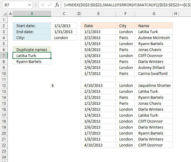
Thank you for your awesome formula, its a bit too advanced for me to be honest but I do grasp the concept of it. I would like to ask you is it possible to encapsulate the formula in an if statement somehow? or as it is in my case "IF from London + IF this month + then PULL unique agent names" I did give it a try but the formula could not work :(
Thanks in advance!
Best Regards,
FB
Neophyte,
Read this:
Extract duplicates using conditions
Huge thank you for your fast response however this is truly outside my league :D (our office excel guru's league too as it seems)... I am trying to pull the "Unique" names rather than duplicates and I don't understand your formula in order to reverse it.
Any help on the subject will be highly appreciated!
THANK YOU!
Neophyte,
Array formula in cell A6:
Get the Excel *.xlsx file
Extract-duplicates-using-conditions_ver2.xlsx
The formulas can be smaller if you have space for a "helper column" in your sheet. The dates make the formulas complicated.
Hi Oscar
Extract a list of duplicates from a column using array formula, does not work for me ? I am using Ms Office 2012
Julio,
did you create an array formula?
Hi, very useful info here.. I can't seem to leave a comment on previous post "How to extract a unique distinct list from a column in excel" so i posted a reply to this thread instead. Sorry..
Anyways, my problem is I wanted to get the unique list only if one condition in one cell is True (Column B). I tried using if() statement but i guess there's something wrong. I know it's very easy for you.. Tnx a lot for your help.
Ex:
A B
1111 True
1232 False
1234 True
Lester,
Read this, I think it is what you are looking for.
Thanks a lot Oscar for your help... Just what i needed... :))
I said before that you're a genius
But I want the previous version (office 2003)
I said before that you're a genius
But I want the previous formula (office 2003)
Hi Oscar,
I am using the unique formula you created in response to Neophyte in the comment above. However, I would like to copy the formula across instead of down. How would I modify the formula to accomplish this?
Thank you for the help!
Kyle
Hi Oscar,
Disregard my last question. I figured it out. I just changed the last row formula to column and it worked.
Thanks,
Kyle
How to convert(transpose) sing column to row.
Thanks,
Chethan kumar
How to convert(transpose) single column to row.
Thanks,
Chethan kumar
Reply
Hi,
Just wondering if I would use this formula to return a list so it would show all duplicates as one, and single entries as they are
ie This List: Green, Yellow, Red, Yellow, Blue, Black, Green, Yellow, Oragne, Blue, Green, Pink
To A list like this: Green, Yellow, Red, Blue, Black, Orange, Pink
Thanks
Got it, not to worry.
Hi Oscar,
I am having issues with the listing formula, I have a table as below:
S.no Month Date Session Name Session Duration Trainer
1 Sep 05-Sep-14 The Art of Tactful conversations 0.5 ABC
2 Sep 09-Sep-14 Managing Client Expectations 0.5 DEF
3 Sep 11-Sep-14 Creativity and Lateral Thinking 0.5 SBC
4 Sep 15 Sep14 and 16 Sep Shaping Customer Agenda 2 days ABC
5 Sep 16-Sep-14 The Art of Presentation Skills 0.5 SBC
6 Sep 23-Sep-14 Happiness @ Work 0.5 ABC
7 Sep 25-Sep-14 Emotional Intelligence 1 day DEF
8 Sep 29-Sep-14 Influencing and Negotiation skills 0.5 DEF
9 Sep 29-Sep-14 Planning and Prioritisation 0.5 SBC
10 Sep 30-Sep-14 Strengthening Workplace relations 0.5 ABC
I need to get a list of trainings done if i update a trainers name.
This has to be done in a seperate workbook.
Please help.
Thanks
DS
Iam trying to add this formula for my work but it doesnt work and it comes up with #Name? Please help
thnx
This function seems to ignore any entry in List1 that has only one entry... Is that correct?
Tried this function using a list from a different sheet in by workbook, for some reason it is listing the results in doubles. Any reason for this? Using Excel 2013.
Nate
Hard to say without seeing your workbook, you entered it as an array formula?
Hi Oscar,
Thanks for your formula, I would like to know how can the duplicate be shown in row and expand to the right? Please help!
Jackie,
(Press with left mouse button to see full size image)
The formula is the same:
=INDEX(List1, MATCH(0, COUNTIF(C1:$C$1, List1)+IF(COUNTIF(List1, List1)>1, 0, 1), 0)) + CTRL + SHIFT + ENTER.
Make sure the cell ref (bolded) is pointing to the next cell to the left, however this means you can't enter the formula in the first column.
I was able to adjust this to my project, but man does it take a long time to calculate. I have a spread sheet with about 4000 rows and it can take hours to calculate. Is there a faster way of doing this?
Hi Oscar, stumbled across this formula and it's quality!!! Your formula nearly works perfectly for me but how do I introduce an exception? Your formula finds and retrieves duplicate tennis players names, however if I wanted to exclude the name "Federer, Roger" from my results how would I do this? The list I am checking for duplicates has some legitimate duplicate text which I need to exclude from the returned results, thanks
Ben,
Thank you!
I have added your question to this post.
Read this: https://www.get-digital-help.com/extract-a-list-of-duplicates-from-a-column-using-array-formula-in-excel/#exceptions
[…] https://www.get-digital-help.com/extract-duplicate-values-with-exceptions/ […]
Hi Oscar,
i've really tried to understand why this formula - as awesome as it is - wouldn't filter triple (etc.) values in list A. If you enter one more Federer in A he appears in E. The version of this kind of formula without the second countif clause (inside the if that kills the unique values) lists anything that comes up more than once just fine, not only duplicates. Now, i've come up with the following formula, which actually seems to work:
=IFERROR(INDEX($A$2:$A$20;MATCH(0;COUNTIF(E1:$E$1;$A$2:$A$20)+IF(COUNTIF($A$2:$A$20;$A$2:$A$20)>1+(COUNTIF($A$2:$A$20;$A$2:$A$20)-COUNTIF($C$2:$C$3;$A$2:$A$20))*COUNTIF($C$2:$C$3;$A$2:$A$20);0;1);0));"")
But i'm no excel expert, and it has a feel of not being the most elegant solution at all... Any ideas? Thanks so much for all the help!
Hi Stephan
Thank you for telling me and thanks for your formula.
This regular formula seems to work as well:
Step 1: Add a new column next to your data-field column, called count
Step 2: insert 1 in the first field and drag-to cover the full length of the data-set so that you have count=1 for all rows
Step 3: insert a pivot table with data-field column and count column
Step 4: drag data-field column header to rows
Step 5: drag count column to values and select SUM() function
Now you can see the data-fields listed on the left side with cardinality against each one of them.
No complex formulas are needed to find repeating values.
Satheesh,
No complex formulas are needed to find repeating values.
I am trying to provide all possible techniques, some people want a formula.
You don't have to add a new column containing 1 in each cell to identify duplicates:
https://www.get-digital-help.com/excel-pivot-tables/#count
Thank you for your comment.
[…] Filter duplicate words from a cell range in excel (udf) […]
Hi
How would i go about just looking if data matched in just one column ?
so get the row extracted based on matching values in column 3?
richard reeves
Try this:
=INDEX($A$2:$D$25, SMALL(IF(COUNTIF($C$2:$C$25,$C$2:$C$25)>1,ROW($A$2:$A$25)-MIN(ROW($A$2:$A$25))+1),ROW(A1)),COLUMN(A1))
My example has only 10 and 11 in column C so all records are extracted. (10 and 11 are duplicates.)
Hi All,
I'm well aware that this article is almost 10yo but I happen to need this exact VBA code (or ideally one that will highlight the duplicate words from several strings texts across a selected range). HoweverI'm having issue getting this to work for me. I keep getting the "Syntax error message".
Any chance someone can help?
Thank you
Hi Ely
I keep getting the "Syntax error message".
The code shown in this article is now working.
Is it possible to list all duplicates using FREQUENCY formula?
The formulas with countif doesn't allow to start from the very first row due to circular reference.
Hi Oscar, I am a fan of your page and your work. I really thank you for helping me a lot. Could you get the duplicate values only once and in turn get unique values? How would you do it? Example I have sheet 1:
column A, column B
dario perez
dario perez
dario arrieta
dario arrieta
dario sandoval
The result recorded in columns c and d would be:
column C, column D
dario perez
dario arrieta
dario sandoval
Thanks!
This formula actually doesn't bring back correct results. If an item is a duplicate but wasn't a result in the prior row it is missing it. I replicated tis formula for my file and tested the results., FYI
Hi, I need little help, I have a data of thousand of customer accounts and their account maintaining branch Code. I have been assigned a task to extract branches list and its accounts details according to the given criteria;
I have to extract all those branches and its accounts where a customer have multiple accounts with one CIF# in same branch, for example A customer has CIF # 1234 in 001 branch (its a branch code) 10 accounts are linked with this CIF# in the same branch and there are 05 other accounts which are linked with this CIF but maintained in other different branches; I have to extract the data branches & the accounts where one CIF has multiple accounts in same branch.
here is my table for sample
Branch Code CIF# A/C#
001 123 001001230002151
001 123 002001230002351
001 123 003000123000546
002 123 004000123000445
Hi Dr,
I excited if you could help me work out how to approach the following challenge:
I have a table with repeated IDs in one columns, and dates of when they were admitted in another.
I need to calculate the time spend measure between two dates for the repeated IDs.
Many thanks direction on this one!
Great work! I've been searching for a couple of hours, and your formula, while intimidating and I don't really understand the logic, works.
I wanted to match just by 1 row in 3 columns B,C,D, so I changed it to the below formula. Just need to figure out how to handle div\0 errors when there is NO duplicate and it would be perfect for me.
=IFERROR(IFERROR(LOOKUP(2, 1/((COUNTIF($E$2:E2, B3)=0)*(COUNTIF(B3, B3)>1)),B3), LOOKUP(2, 1/((COUNTIF($E$2:E2, C3)=0)*((COUNTIF(C3,C3)>1)+(COUNTIF(B3,C3)>0))),C3)),LOOKUP(2, 1/((COUNTIF($E$2:E2,D3)=0)*((COUNTIF(D3, D3)>1)+(COUNTIF(B3, D3)>0)+(COUNTIF(C3, D3)>0))), D3))