Filter unique distinct records
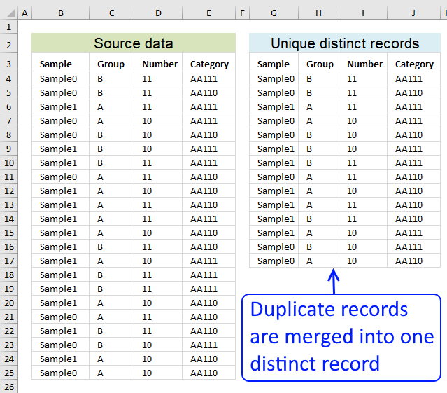
Table of contents
- Filter unique distinct row records
- Filter unique distinct row records but not blanks
- Filter unique distinct row records that does not begin with *string*
- Filter unique distinct row records that begins with *string*
- Filter unique distinct records [Pivot table]
- Filter unique distinct records based on a condition
- Extract unique distinct records based on condition example 2
- Extract unique distinct records from two data sets
- Extract a unique distinct list and sum amounts based on a condition - earlier Excel versions
- Extract a unique distinct list and sum amounts based on a condition - Excel 365
- List all unique distinct rows in a given month and year
- List all unique distinct rows in a given month and year (Excel 365)
- List all rows in a given month and year
- List all rows in a given month and year (Excel 365)
1. How do I extract unique distinct rows?
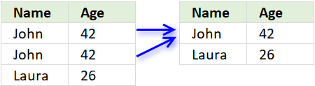
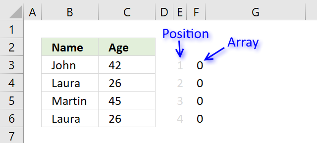
First, let me explain unique distinct records. A record is an entire row in the table, in this example. The picture below displays a small table in columns B and C containing a duplicate record. The table in columns E and F contains unique distinct records only.
In other words, unique distinct records are all records but duplicate records are removed.
Second, I highly recommend using a pivot table to extract unique distinct records if you are working with a really large data set. A Pivot table is incredibly fast and is also easy to quickly set up and manage.
Third, this post shows you how to construct an array formula that extracts unique distinct records.
Update 10 December 2020, Excel 365 formula:
This is a much smaller regular formula, you can read more about the UNIQUE function here: Extract unique distinct rows
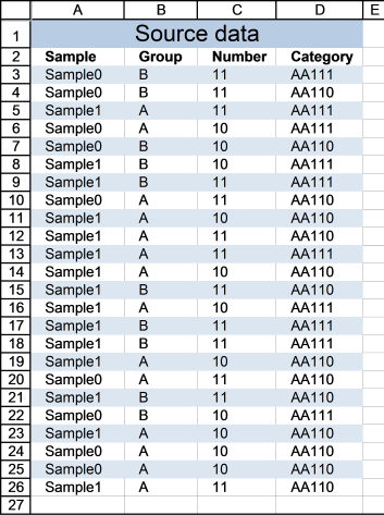
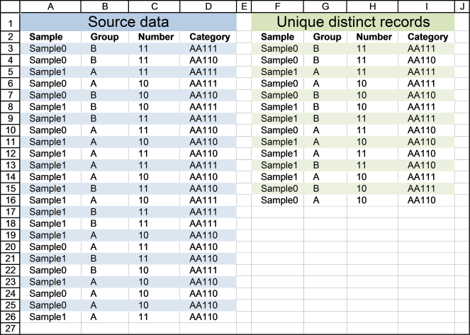
Cell range A3:D26 contains the original list, cell range F3:I16 contains the extracted list. The following formula works for Excel versions prior to Excel 365.
Array formula in cell F3:
How to enter an array formula
- Select cell F3
- Type above formula in cell or formula bar
- Press and hold CTRL + SHIFT simultaneously
- Press Enter once
If you did the steps above correctly, the formula has now a beginning and ending curly bracket, like this {=array_formula}
Don't enter these characters yourself, they appear automatically if you did this right.
How to copy formula
Copy cell F3 and paste it to cells to the right, as far as needed. Then copy cells and paste them down, as far as needed.
Explaining array formula in cell F3
You can easily follow along while I go through this array formula, go to tab "Formulas" on the ribbon. Select cell F3 then press with left mouse button on "Evaluate Formula" button. Press with left mouse button on "Evaluate" button to move to next step.
Step 1 - Identify rows with unique records
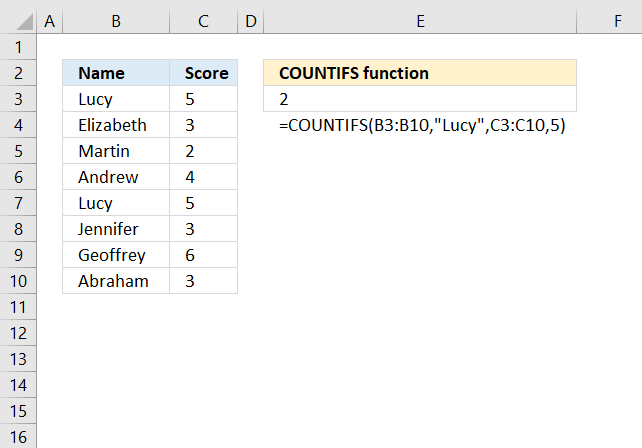
The COUNTIFS function counts the number of cells specified by a given set of conditions or criteria
COUNTIFS($F$2:$F2, $A$3:$A$26, $G$2:$G2, $B$3:$B$26, $H$2:$H2, $C$3:$C$26, $I$2:$I2, $D$3:$D$26)
becomes
COUNTIFS($A$28:$A28, {"Sample0"; "Sample0"; "Sample1"; "Sample0"; "Sample0"; "Sample1"; "Sample1"; "Sample0"; "Sample1"; "Sample1"; "Sample1"; "Sample1"; "Sample1"; "Sample1"; "Sample1"; "Sample1"; "Sample1"; "Sample0"; "Sample1"; "Sample0"; "Sample1"; "Sample0"; "Sample0"; "Sample1"}, $B$28:$B28, {"B";"B";"A";"A";"B";"B"; "B";"A";"A";"A";"A";"A";"B";"A";"B"; "B";"A";"A";"B";"B";"A";"A";"A";"A"}, $C$28:$C28, {11; 11; 11; 10; 10; 10; 11; 11; 10; 11; 11; 10; 11; 10; 11; 11; 10; 11; 11; 10; 10; 10; 10; 11}, $D$28:$D28, {"AA111"; "AA110"; "AA111"; "AA111"; "AA110"; "AA111"; "AA111"; "AA110"; "AA110"; "AA110"; "AA111"; "AA110"; "AA110"; "AA111"; "AA111"; "AA111"; "AA110"; "AA110"; "AA110"; "AA111"; "AA110"; "AA110"; "AA110"; "AA110"})
becomes
COUNTIFS("Sample", {"Sample0"; "Sample0"; "Sample1"; "Sample0"; "Sample0"; "Sample1"; "Sample1"; "Sample0"; "Sample1"; "Sample1"; "Sample1"; "Sample1"; "Sample1"; "Sample1"; "Sample1"; "Sample1"; "Sample1"; "Sample0"; "Sample1"; "Sample0"; "Sample1"; "Sample0"; "Sample0"; "Sample1"}, "Group", {"B";"B";"A";"A";"B";"B"; "B";"A";"A";"A";"A";"A";"B";"A";"B"; "B";"A";"A";"B";"B";"A";"A";"A";"A"}, "Number", {11; 11; 11; 10; 10; 10; 11; 11; 10; 11; 11; 10; 11; 10; 11; 11; 10; 11; 11; 10; 10; 10; 10; 11}, "Category", {"AA111"; "AA110"; "AA111"; "AA111"; "AA110"; "AA111"; "AA111"; "AA110"; "AA110"; "AA110"; "AA111"; "AA110"; "AA110"; "AA111"; "AA111"; "AA111"; "AA110"; "AA110"; "AA110"; "AA111"; "AA110"; "AA110"; "AA110"; "AA110"})
and returns
{0; 0; 0; 0; 0; 0; 0; 0; 0; 0; 0; 0; 0; 0; 0; 0; 0; 0; 0; 0; 0; 0; 0; 0}
Step 2 - Find relative position of a unique record
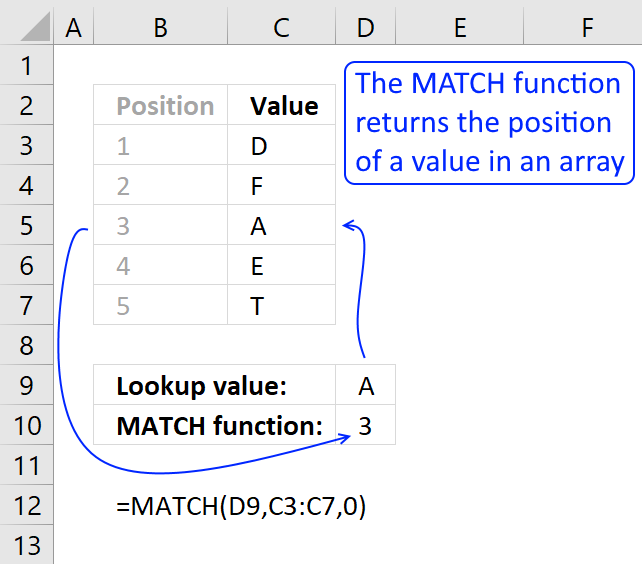
The MATCH function returns the relative position of an item in an array that matches a specified value
MATCH(0, COUNTIFS($F$2:$F2, $A$3:$A$26, $G$2:$G2, $B$3:$B$26, $H$2:$H2, $C$3:$C$26, $I$2:$I2, $D$3:$D$26), 0)
becomes
MATCH(0, {0; 0; 0; 0; 0; 0; 0; 0; 0; 0; 0; 0; 0; 0; 0; 0; 0; 0; 0; 0; 0; 0; 0; 0}, 0)
and returns 1.
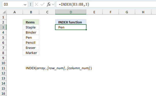
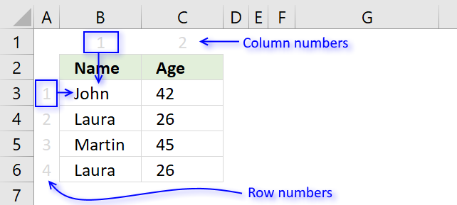
Step 3 - Return a value of the cell at the intersection of a particular row and column
The INDEX function returns a value or reference of the cell at the intersection of a particular row and column, in a given range
INDEX($A$3:$D$26, MATCH(0, COUNTIFS($F$2:$F2, $A$3:$A$26, $G$2:$G2, $B$3:$B$26, $H$2:$H2, $C$3:$C$26, $I$2:$I2, $D$3:$D$26), 0), COLUMN(A1))
becomes
INDEX($A$3:$D$26, 1, COLUMN(A1))
becomes
INDEX($A$3:$D$26, 1, 1)
becomes
INDEX({"Sample0", "B", 11, "AA111"; "Sample0", "B", 11, "AA110"; "Sample1", "A", 11, "AA111"; "Sample0", "A", 10, "AA111"; "Sample0", "B", 10, "AA110"; "Sample1", "B", 10, "AA111"; "Sample1", "B", 11, "AA111"; "Sample0", "A", 11, "AA110"; "Sample1", "A", 10, "AA110"; "Sample1", "A", 11, "AA110"; "Sample1", "A", 11, "AA111"; "Sample1", "A", 10, "AA110"; "Sample1", "B", 11, "AA110"; "Sample1", "A", 10, "AA111"; "Sample1", "B", 11, "AA111"; "Sample1", "B", 11, "AA111"; "Sample1", "A", 10, "AA110"; "Sample0", "A", 11, "AA110"; "Sample1", "B", 11, "AA110"; "Sample0", "B", 10, "AA111"; "Sample1", "A", 10, "AA110"; "Sample0", "A", 10, "AA110"; "Sample0", "A", 10, "AA110"; "Sample1", "A", 11, "AA110"}, 1, 1)
and returns "Sample0" in cell F3.
Related articles
Recommended articles

First, let me explain the difference between unique values and unique distinct values, it is important you know the difference […]
2. Filter unique distinct row records but not blanks
The image below shows you a data table in column A:D. Unfortunately, it has some blank rows, however, the formula below takes handles this issue.
![]()
Update 11 December 2020, Excel 365 formula in cell F3:
This is a much smaller formula also entered as a regular formula, you can read more about the UNIQUE function here: Extract unique distinct rows ignoring blank rows
The following array formula in cell F3 works with previous Excel versions:
3. Extract unique distinct rows that don't begin with a given string
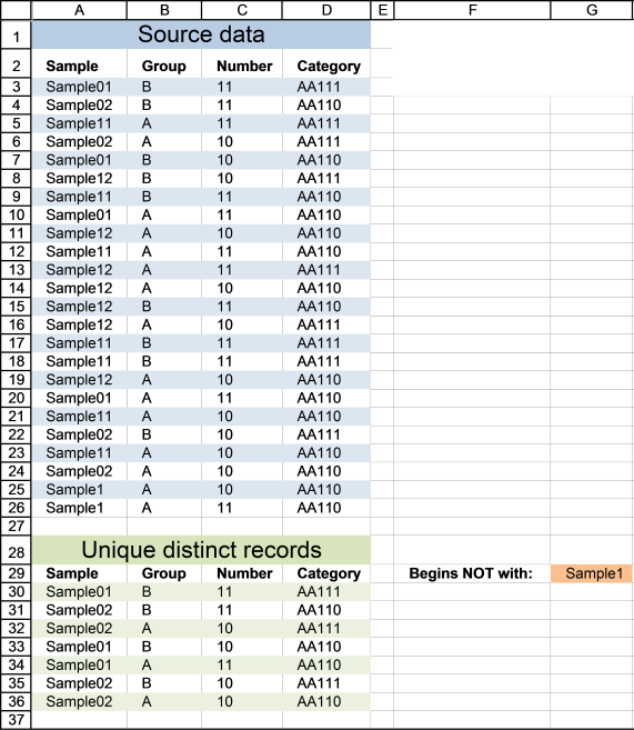
This example lets you specify a string and a record is shown in cell range A30:D36 if it does NOT match the beginning characters in column A and it is NOT a DUPLICATE record.
Update 11 December 2020, Excel 365 formula in cell A30:
The formula below is for previous Excel versions.
Array formula in cell A30:
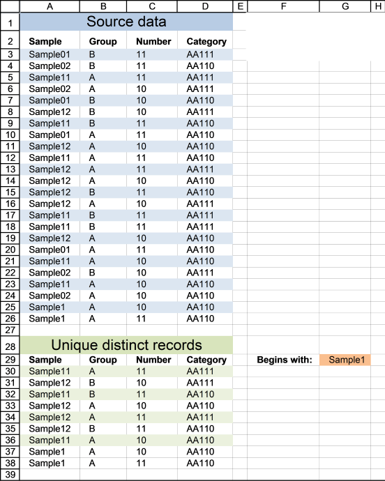
4. Extract unique distinct rows that begin with *string*
If you are looking for records that begin with *string*, see this formula. Note that the formula looks for values in col A that begins with a specific text string.
Update 11 December 2020, Excel 365 formula in cell A30:
The formula below is for previous Excel versions.
Array formula in cell A30:
6. Filter unique distinct records with a condition

If Tea and Coffee has Americano,it will only return Americano once and not twice. I am looking for a unique distinct list based on each condition.
I remember reading that Excel has difficulty with these type of or conditions in arrays.
Answer:
Array formula in cell C19:
To enter an array formula, type the formula in a cell then press and hold CTRL + SHIFT simultaneously, now press Enter once. Release all keys.
The formula bar now shows the formula with a beginning and ending curly bracket telling you that you entered the formula successfully. Don't enter the curly brackets yourself.
Excel 365 dynamic array formula in cell C19:
Copy array formula
- Select cell C19
- Copy cell (Ctrl + c)
- Select cell range C19:D22
- Paste (Ctrl + v)
How the array formula in cell C19 works
Step 1 - Identify unique distinct records
COUNTIFS($C$18:C18, $C$5:$C$11, $D$18:D18, $D$5:$D$11)
becomes
COUNTIFS("Category", {"Coffee";"Coffee";"Coffee";"Coffee";"tea";"juice";"tea"}, "Item", {"Espresso";"Espresso";"Americano";"Americano";"Americano";"Florida";"English"},)
and returns {0;0;0;0;0;0;0}
Recommended articles
Checks multiple conditions against the same number of cell ranges and counts how many times all criteria are met.
Step 2 - Filter records with condition
COUNTIF($C$13:$C$14, $C$5:$C$11)=0
becomes
COUNTIF({"Coffee"; "tea"}, {"Coffee"; "Coffee"; "Coffee"; "Coffee"; "tea"; "juice"; "tea"})=0
and returns {FALSE; FALSE; FALSE; FALSE; FALSE; TRUE; FALSE}
Recommended articles

Counts the number of cells that meet a specific condition.
Step 3 - Match filtered records
MATCH(0, COUNTIFS($C$18:C18, $C$5:$C$11, $D$18:D18, $D$5:$D$11)+(COUNTIF($C$13:$C$14, $C$5:$C$11)=0), 0)
becomes
MATCH(0, {0;0;0;0;0;0;0}+{FALSE; FALSE; FALSE; FALSE; FALSE; TRUE; FALSE}, 0)
becomes
MATCH(0, {0;0;0;0;0;1;0},0)
and returns 1.
Recommended articles
Identify the position of a value in an array.
Step 4 - Return a value or reference of the cell at the intersection of a particular row and column
INDEX($C$5:$D$11, MATCH(0, COUNTIFS($C$18:C18, $C$5:$C$11, $D$18:D18, $D$5:$D$11)+(COUNTIF($C$13:$C$14, $C$5:$C$11)=0), 0), COLUMN(A1))
becomes
INDEX({"Coffee", "Espresso";"Coffee", "Espresso";"Coffee", "Americano";"Coffee", "Americano";"tea", "Americano";"juice", "Florida";"tea", "English"}, 1, 1)
and returns "Coffee" in cell C19.
Recommended articles
Gets a value in a specific cell range based on a row and column number.
Tip! Did you know that a pivot table can easily extract unique distinct records too?
Recommended articles
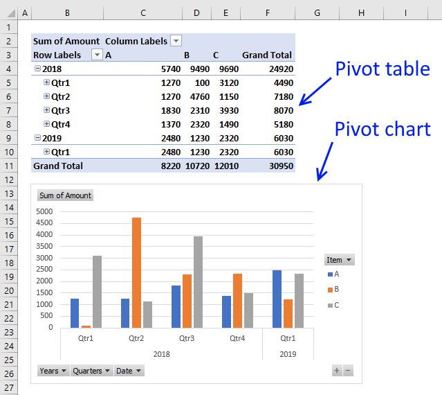
A pivot table allows you to examine data more efficiently, it can summarize large amounts of data very quickly and is very easy to use.
How to remove errors
IFERROR(value, value_if_error) returns value_if_error if expression is an error and the value of the expression itself otherwise
The array formula becomes:
7. Extract unique distinct records based on condition, example 2
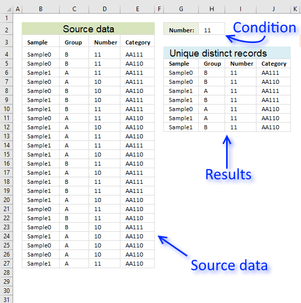
In this section, I want to show you how to narrow that search down a bit further. This time I want to search for unique distinct records based on a condition that must match. I want to extract for unique distinct records with column C containing value 11.
Array formula in G6:
To enter an array formula, type the formula in cell G6 then press and hold CTRL + SHIFT simultaneously, now press Enter once. Release all keys.
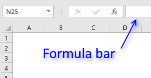 The formula bar now shows the formula with a beginning and ending curly bracket telling you that you entered the formula successfully.
Don't enter the curly brackets yourself, they appear automatically.
Excel 365 dynamic array formula in cell G6:
Explaining formula in cell G6
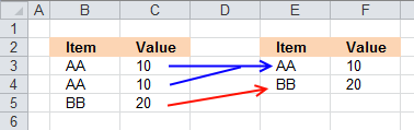
First, let me explain what a unique distinct record is. A record is an entire row in the table, in this example. The picture below displays a small table in column B and C containing a duplicate record. The table in column E and F contains only unique distinct records.
In other words, unique distinct records are all records but duplicate records are removed. The record in cell range B4:C4 is removed.
Step 1 - Check if records have been displayed
The COUNTIFS function lets you count values combined which is perfect when it comes to counting data records. The following part of the formula checks if previous records in the list has been displayed, if a record has been shown the corresponding value in the array returns 1 and if not 0 (zero).
COUNTIFS($G$5:$G5, $B$4:$B$27, $H$5:$H5, $C$4:$C$27, $I$5:$I5, $D$4:$D$27, $J$5:$J5, $E$4:$E$27)
returns {0; 0; 0; 0; 0; 0; 0; 0; 0; 0; 0; 0; 0; 0; 0; 0; 0; 0; 0; 0; 0; 0; 0; 0}.
This means that no record has been displayed yet in the list, remember that we are checking the formula in cell G6.
Step 2 - Make sure that only records with the condition met are filtered
The COUNTIF function lets you build an array that indicates which records meet the condition.
COUNTIF($H$2,$D$4:$D$27)=0
becomes
{1;1;1;0;0;0;1;1;0;1;1;0;1;0;1;1;0;1;1;0;0;0;0;1}=0
and returns {FALSE; FALSE; FALSE; TRUE; TRUE; TRUE; FALSE; FALSE; TRUE; FALSE; FALSE; TRUE; FALSE; TRUE; FALSE; FALSE; TRUE; FALSE; FALSE; TRUE; TRUE; TRUE; TRUE; FALSE}.
Step 3 - Add arrays
COUNTIFS($G$5:$G5, $B$4:$B$27, $H$5:$H5, $C$4:$C$27, $I$5:$I5, $D$4:$D$27, $J$5:$J5, $E$4:$E$27)+(COUNTIF($H$2,$D$4:$D$27)=0)
becomes
{0; 0; 0; 0; 0; 0; 0; 0; 0; 0; 0; 0; 0; 0; 0; 0; 0; 0; 0; 0; 0; 0; 0; 0} + {FALSE; FALSE; FALSE; TRUE; TRUE; TRUE; FALSE; FALSE; TRUE; FALSE; FALSE; TRUE; FALSE; TRUE; FALSE; FALSE; TRUE; FALSE; FALSE; TRUE; TRUE; TRUE; TRUE; FALSE}
and returns {0;0;0;1;1;1;0;0;1;0;0;1;0;1;0;0;1;0;0;1;1;1;1;0}.
Step 4 - Find the position of the first 0 (zero) in the array
To be able to get the record we need the formula needs to know where the first record is that not yet has been shown. The MATCH function lets you find the position of the first 0 (zero) in the array.
MATCH(0, COUNTIFS($G$5:$G5, $B$4:$B$27, $H$5:$H5, $C$4:$C$27, $I$5:$I5, $D$4:$D$27, $J$5:$J5, $E$4:$E$27)+(COUNTIF($H$2,$D$4:$D$27)=0), 0)
becomes
MATCH(0, {0;0;0;1;1;1;0;0;1;0;0;1;0;1;0;0;1;0;0;1;1;1;1;0}, 0)
and returns 1.
Step 5 - Return the first value from the first record
The INDEX function lets you get a value from the worksheet based on a row number and column number.
INDEX($B$4:$E$27, MATCH(0, COUNTIFS($G$5:$G5, $B$4:$B$27, $H$5:$H5, $C$4:$C$27, $I$5:$I5, $D$4:$D$27, $J$5:$J5, $E$4:$E$27)+(COUNTIF($H$2,$D$4:$D$27)=0), 0), COLUMN(A1))
becomes
INDEX($B$4:$E$27, 1, COLUMN(A1))
becomes
INDEX($B$4:$E$27, 1, 1)
and returns "Sample0" in cell G6.
Get Excel *.xlsx file
Extract unique distinct records based on a condition.xlsx
8. Extract unique distinct records from two data sets
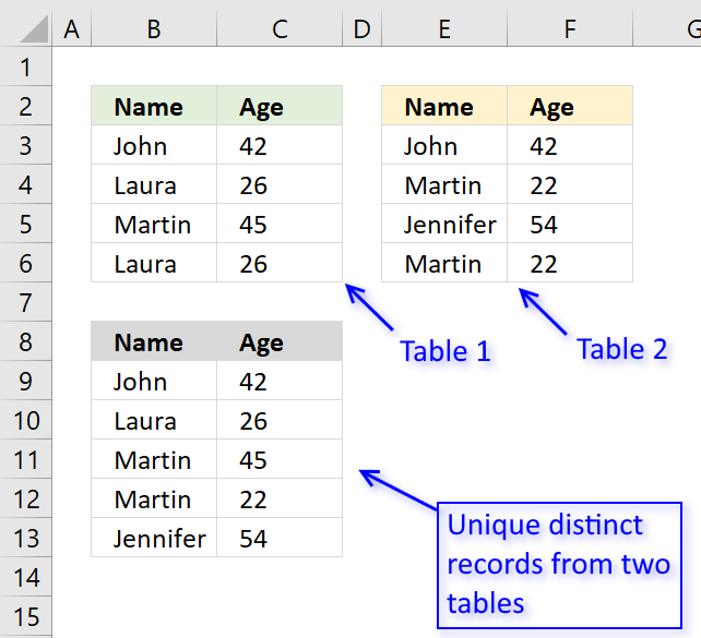
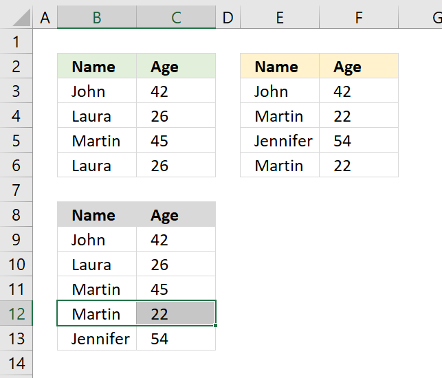
The picture above shows an array formula in cell B9:C13 that extracts unique distinct records from two tables in cell range B3:C6 and E3:F6.
If a record exists in both tables only one record is returned by the formula. If a record exists multiple times in one table only one record is returned by the formula.
Example, John 42 exists in both tables, however, the formula returns only one instance of John 42.
Laura 26 exists multiple times but only in the first table, the formula returns only one record of Laura 26.
Excel 365 dynamic array formula in cell B9:
Array formula in cell B9 for older Excel versions:
To enter an array formula, type the formula in cell B9 then press and hold CTRL + SHIFT simultaneously, now press Enter once. Release all keys.
The formula bar now shows the formula with a beginning and ending curly bracket telling you that you entered the formula successfully.
Don't enter the curly brackets yourself, they appear automatically.
What is a unique distinct record?
Unique distinct records are all records except duplicates merged into one distinct value.
In other words, duplicate records are removed.
Explaining the formula in cell B9
Use the "Evaluate Formula" tool to examine the calculation steps in greater detail.
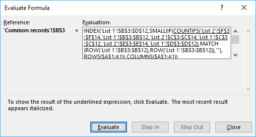 Go to tab "Formula" on the ribbon, press with left mouse button on "Evaluate Formula" button to start the tool.
Then press with left mouse button on the "Evaluate" button to see the next step in the calculation, this will make it easier to understand how the formula works.
Step 1 - Count previous records against table 1
The COUNTIFS function allows you to count how many times a record exists in a table.
The previous values in cell B9 are the values in B8 and C8.
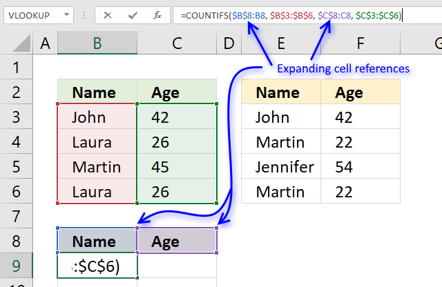
The first argument $B$8:B8 in the COUNTIFS function has both absolute and relative cell references, this allows the formula to automatically expand when you copy it and paste to cells below.
"Name" and "Age" is not found in cell range B3:C6 so the COUNTIFS function returns 0 (zero) for each record.
COUNTIFS($B$8:B8, $B$3:$B$6, $C$8:C8, $C$3:$C$6)
becomes
=COUNTIFS("Name", {"John";"Laura";"Martin";"Laura"}, "Age", {42;26;45;26})
and returns {0;0;0;0}. There are four records and the function returns an array containing 4 values (zeros).
Step 2 - Find the first instance of 0 (zero) in the array
The MATCH function allows you to identify which record to return next.
MATCH(0, COUNTIFS($B$8:B8, $B$3:$B$6, $C$8:C8, $C$3:$C$6), 0)
becomes
MATCH(0, {0;0;0;0}, 0)
and returns 1. The first instance of 0 (zero) is found in position 1 in the array.
Step 3 - Return value from a record
The INDEX function lets get a specific value using a row and column number.
The MATCH function calculates the row number we need to get the correct value, however, the COLUMNS function keeps track of which value in the record to get.
The COLUMNS function calculates the number of columns in a cell reference, the cell reference used here $A$1:A1 is also expanding when the formula is copied to other cells.
COLUMNS($A$1:A1) returns 1.
INDEX($B$3:$C$6, MATCH(0, COUNTIFS($B$8:B8, $B$3:$B$6, $C$8:C8, $C$3:$C$6), 0),COLUMNS($A$1:A1))
becomes
INDEX($B$3:$C$6, 1, COLUMNS($A$1:A1))
becomes
INDEX($B$3:$C$6, 1, 1) and returns John in cell B9.
Step 4 - IFNA function points the calculation in a new direction
Step 1 to 3 explains how the formula extracts unique distinct records from the first table.
The first part of the formula returns a #N/A error when there are no records left in table 1 to extract.
The IFNA function points the calculation to part2 when the error occurs.
The second part of the formula does the exact same thing as the first part except that the cell references this time points to the second table.
The picture above shows that the two last records are extracted from the second table.
Get Excel *.xlsx file
Extract unique distinct records from two data sets.xlsx
9. Extract a unique distinct list and sum amounts based on a condition - earlier Excel versions
Anura asks:
Is it possible to extend this by matching items that meet a criteria?
I have a list of credit card transactions showing the name of the card holder, their Branch and the amount. I want to produce a report for each Branch, so what I want is to extract only those people who match the Branch name. For example:
Frank Branch A
Frank Branch A
Frank Branch A
Joe Branch A
Mary Branch B
Jane Branch C
Mike Branch A
Joe Branch A
Dave Branch C
I would like a list of only those people for Branch A, and then be able to summarise the transactions. Or should I do this in two stages?
Answer:
This post demonstrates how to build a formula to extract a unique distinct list using a condition, however, I highly recommend a pivot table for this task: Pivot table - Unique distinct list
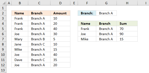
Type a branch in cell G2 and the formulas in cell range F5:H7 returns the correct records from B3:D12. If you have more than two values in one record (except the number) use the COUNTIFS function to filter unique distinct records.
Array formula in F5:
Copy cell F5 and paste to cell range F5:G7.
Formula in cell H5:
If you have a version earlier than Excel 2007 use the SUMPRODUCT function
If you are interested in how the SUMPRODUCT function works, read:
Recommended articles
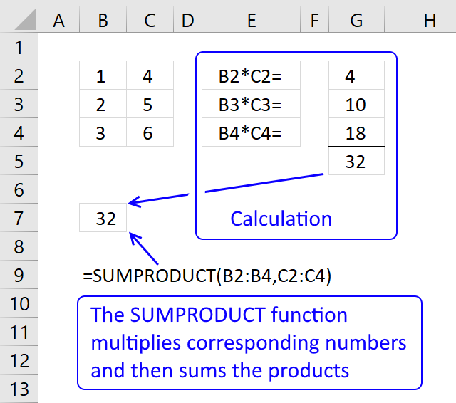
The SUMPRODUCT function calculates the product of corresponding values and then returns the sum of each multiplication.
Watch a video where I explain the formula
Recommended link
Recommended articles
First, let me explain the difference between unique values and unique distinct values, it is important you know the difference […]
How to enter an array formula
- Copy (Ctrl + c) above formula
- Double press with left mouse button on cell E8
- Paste (Ctrl + v) to cell
- Press and hold CTRL + Shift simultaneously
- Press Enter
- Release all keys
Copy cell E8 and paste it down as far as needed. Copy cells and paste into cell range F8 and down as far as needed.
Recommended link
Recommended articles

Array formulas allows you to do advanced calculations not possible with regular formulas.
Explaining array formula in cell E8
Step 1 - Check previous values to make sure they are not repeated
COUNTIF($E$7:$E7, $A$2:$A$11)
If you examine the cell references you may find this strange: $E$7:$E7 It is an absolute and relative cell reference. It expands when the formula is copied across the spreadsheet. Read more here: Absolute and relative references in excel
COUNTIF($E$7:$E7, $A$2:$A$11)
returns {0;0;0;0;0;0;0;0;0;0}
Step 2 - Compare values in column B with the value in cell F1
($B$2:$B$11<>$F$1)
returns {FALSE; ... ; FALSE}
Step 3 - Add arrays
COUNTIF($E$7:$E7, $A$2:$A$11)+($B$2:$B$11<>$F$1)
becomes
{0;0;0;0;0;0;0;0;0;0} + {FALSE; FALSE; FALSE; FALSE; TRUE; TRUE; FALSE; FALSE; TRUE; FALSE}
and returns
{0;0;0;0;1;1;0;0;1;0}
Step 4 - Find first 0 (zero) in array
MATCH(0, COUNTIF($E$7:$E7, $A$2:$A$11)+($B$2:$B$11<>$F$1), 0)
becomes
MATCH(0, {0;0;0;0;1;1;0;0;1;0}, 0)
and returns 1.
Step 5 - Return a value or reference of the cell at the intersection of a particular row and column
INDEX($A$2:$C$11, MATCH(0, COUNTIF($E$7:$E7, $A$2:$A$11)+($B$2:$B$11<>$F$1), 0), COLUMN(A1))
returns "Frank" in cell E8.
Get Excel *.xls file
unique distinct list matching criteria.xls
(Excel 97-2003 Workbook *.xls)
10. Extract a unique distinct list and sum amounts based on a condition - Excel 365

The following dynamic Excel 365 formula aggregates or groups the amounts based "Name" and the specified "Branch" in cell C14, and then sorts the output array based on the amounts.
The image above shows this data table in cell range B2:D12:
| Name | Branch | Amount |
| Frank | Branch A | 10 |
| Frank | Branch A | 20 |
| Frank | Branch A | 40 |
| Joe | Branch A | 30 |
| Mary | Branch B | 5 |
| Jane | Branch C | 10 |
| Mike | Branch A | 15 |
| Joe | Branch A | 40 |
| Dave | Branch C | 35 |
| Joe | Branch A | 20 |
Formula in cell B17:
The formula in cell B17 returns this dynamic array:
| Joe | Branch A | 90 |
| Frank | Branch A | 70 |
| Mike | Branch A | 15 |
It contains only data based on the specified "Branch" in cell C14 which is "Branch A" in this example. "Branch A" has the following names: Joe, Frank, and Mike and the corresponding amounts are 90, 70, and 15.
Here's a breakdown of the formula:
- SUMIFS(D3:D12,C3:C12,C3:C12,B3:B12,B3:B12): This function calculates the sum of values in column D for each row where the values in columns C and B match the values in the same row. It's essentially a self-referential sumifs that sums up the values in column D for each unique combination of values in columns C and B.
- HSTACK(B3:C12,SUMIFS(...)): This function horizontally stacks (or combines) the values in columns B and C with the results of the sumifs function. This creates a new array with the values from columns B and C, and the corresponding sumifs results.
- FILTER(HSTACK(...),C3:C12=C14): This function filters the array created by the hstack function to only include rows where the value in column C matches the value in cell C14.
- UNIQUE(FILTER(...)): This function removes any duplicate rows from the filtered array, leaving only unique combinations of values.
- SORT(UNIQUE(...),3,-1): This function sorts the unique array in descending order (due to the -1) based on the values in the third column which is the sumifs results.
10.1 Explaining formula
Step 1 - Filter data based on given branch
The SUMIFS function adds numbers based on criteria.
Function syntax: SUMIFS(sum_range, criteria_range1, criteria1, [criteria_range2], [criteria2], ...)
SUMIFS(D3:D12,C3:C12,C3:C12,B3:B12,B3:B12)
returns

Step 2 - Stack arrays horizontally
The HSTACK function combines cell ranges or arrays. Joins data to the first blank cell to the right of a cell range or array (horizontal stacking)
Function syntax: HSTACK(array1,[array2],...)
HSTACK(B3:C12,SUMIFS(D3:D12,C3:C12,C3:C12,B3:B12,B3:B12))
returns

Step 3 - Filter data based on given branch
The FILTER function extracts values/rows based on a condition or criteria.
Function syntax: FILTER(array, include, [if_empty])
FILTER(HSTACK(B3:C12,SUMIFS(D3:D12,C3:C12,C3:C12,B3:B12,B3:B12)),C3:C12=C14)
returns

Step 4 - List unique distinct rows
The UNIQUE function returns a unique or unique distinct list.
Function syntax: UNIQUE(array,[by_col],[exactly_once])
UNIQUE(FILTER(HSTACK(B3:C12,SUMIFS(D3:D12,C3:C12,C3:C12,B3:B12,B3:B12)),C3:C12=C14))
returns

Step 5 - Sort array in descending order based on amounts in column 3
The SORT function sorts values from a cell range or array
Function syntax: SORT(array,[sort_index],[sort_order],[by_col])
SORT(UNIQUE(FILTER(HSTACK(B3:C12,SUMIFS(D3:D12,C3:C12,C3:C12,B3:B12,B3:B12)),C3:C12=C14)),3,-1)
returns
11. List all unique distinct rows in a given month

Question:
I have a table with four columns, Date, Name, Level, and outcome. The range is from row 3 to row 1000.
What I need to be able to do is look at today's date. Determine the month and year and then look up all the values in the date column that match the month and year. I've been trying to get it to work with sumproduct but I can't wrap my head around it.
Then on a separate tab list all the unique events for that month.
So one the separate tab it would show something like this:
May 2/2010 Bob Smith 3 Requires Attention
May 5/2010 Jim Smith 1 Out of Service
Hope you are able to help. Thanks in advance.
Answer:
Array formula in A23:
Copy cell and paste it to the right to D23. Copy A23:D23 and paste it down as far as needed.
11.1 How to create an array formula
- Select cell A23
- Copy/Paste array formula to the formula bar
- Press and hold Ctrl + Shift
- Press Enter
11.2 Explaining array formula in cell A23
Step 1 - Find matching months and years
The DATE function creates an Excel date based on year, month, and day value. The YEAR function returns the year from an Excel date. The MONTH function returns a number representing the position of a given month in a year, based on an Excel date.
DATE(YEAR($C$2), MONTH($C$2), 1)=DATE(YEAR($A$5:$A$9), MONTH($A$5:$A$9), 1))
becomes DATE(2010, 5, 1)=DATE({2010; 2010; 2010; 2010; 2010}, {4; 4; 5; 5; 5}), 1))
becomes 40299={40269; 40269; 40299; 40299; 40299}
and returns {FALSE; FALSE; TRUE; TRUE; TRUE}
Step 2 - Find unique distinct records
This COUNTIFS function prevents duplicate records. It uses absolute and relative cell references in order to create expanding cell references, they grow as the cell is copied to cells below.
COUNTIFS($A$22:$A22, $A$5:$A$9, $B$22:$B22, $B$5:$B$9, $C$22:$C22, $C$5:$C$9, $D$22:$D22, $D$5:$D$9)
returns
{0; 0; 0; 0; 0}
Step 3 - Add arrays
The NOT function returns the boolean opposite, TRUE becomes FALSE and FALSE becomes TRUE.
By adding the arrays we get OR logic meaning at least one value must be TRUE for the result to be TRUE, remember that it is evaluated row-wise.
NOT(DATE(YEAR($C$2), MONTH($C$2), 1)=DATE(YEAR($A$5:$A$9), MONTH($A$5:$A$9), 1))+COUNTIFS($A$22:$A22, $A$5:$A$9, $B$22:$B22, $B$5:$B$9, $C$22:$C22, $C$5:$C$9, $D$22:$D22, $D$5:$D$9)
returns {1; 1; 0; 0; 0}.
Step 4 - Find first unique distinct row in range
The MATCH function returns the relative position of a specific value in an array.
MATCH(0, NOT(DATE(YEAR($C$2), MONTH($C$2), 1)=DATE(YEAR($A$5:$A$9), MONTH($A$5:$A$9), 1))+COUNTIFS($A$22:$A22, $A$5:$A$9, $B$22:$B22, $B$5:$B$9, $C$22:$C22, $C$5:$C$9, $D$22:$D22, $D$5:$D$9), 0)
becomes MATCH(0, {1;1;0;0;0}, 0) and returns 3.
Step 5 - Return a value of the cell at the intersection of a particular row and column
The INDEX function returns a value from a given cell range based on a row and column number.
INDEX($A$5:$D$9, MATCH(0, NOT(DATE(YEAR($C$2), MONTH($C$2), 1)=DATE(YEAR($A$5:$A$9), MONTH($A$5:$A$9), 1))+COUNTIFS($A$22:$A22, $A$5:$A$9, $B$22:$B22, $B$5:$B$9, $C$22:$C22, $C$5:$C$9, $D$22:$D22, $D$5:$D$9), 0), COLUMN(A1))
returns 2-MAy-2010
IFERROR converts errors to blank cells.
12. List all unique distinct rows in a given month (Excel 365)
Dynamic array formula in cell A23:
12.1 How to enter a dynamic array formula
The dynamic array formula is a new feature available in Excel 365, you enter it as a regular formula.
12.2 Explaining dynamic array formula
Step 1 - Calculate number representing the position of the month
The MONTH function returns a number representing the position of a given month in a year, based on an Excel date.
MONTH(serial)
MONTH(B2)
becomes
MONTH(40303)
and returns 5. The fifth month is May.
Step 2 - Compare month numbers to given month
The equal sign lets you compare month numbers to identify dates matching the month, the result is a boolean value.
MONTH(B2)=MONTH(A5:A9)
becomes
5={4; 4; 5; 5; 5}
and returns {FALSE; FALSE; TRUE; TRUE; TRUE}.
Step 3 - Extract year from date
The YEAR function returns the year from an Excel date.
YEAR(serial)
YEAR(B2)
becomes
YEAR(40303)
and returns 2010.
Step 4 - Compare year numbers to the condition
YEAR(B2)=YEAR(A5:A9)
becomes
2010={2010; 2010; 2010; 2010; 2010}
and returns {TRUE; TRUE; TRUE; TRUE; TRUE}.
Step 5 - AND logic
Both tests must be true and to do that we need to multiply the array, in other words, apply AND logic.
Use the asterisk * to multiply values or arrays.
The AND logic behind this is that
TRUE * TRUE = TRUE (1)
TRUE * FALSE = FALSE (0)
FALSE * FALSE = FALSE (0)
(MONTH(B2)=MONTH(A5:A9))*(YEAR(B2)=YEAR(A5:A9))
returns {0; 0; 1; 1; 1}.
Step 6 - Filter values based on array
The FILTER function lets you extract values/rows based on a condition or criteria.
FILTER(array, include, [if_empty])
FILTER(A5:D9, (MONTH(B2)=MONTH(A5:A9))*(YEAR(B2)=YEAR(A5:A9)))
becomes
FILTER(A5:D9, {0; 0; 1; 1; 1})
and returns
{40300, " Bob Smith", ... , "Requires Attention"}.
Step 7 - Extract unique distinct rows/records
The UNIQUE function lets you extract both unique and unique distinct values and also compare columns to columns or rows to rows.
UNIQUE(FILTER(A5:D9, (MONTH(B2)=MONTH(A5:A9))*(YEAR(B2)=YEAR(A5:A9))))
returns {40300, ..., "Out of Service"}.
13. List all rows in a given month and year
The array formula in cell A14 returns all rows that match the month and year from the specified date in cell C2.
Array formula in A14:
Copy cell and paste it to the right to D14. Copy A14:D14 and paste it down as far as needed.
14. List all rows in a given month and year (Excel 365)
The dynamic array formula in cell A14 returns all rows that match the month and year from the specified date in cell C2.
Dynamic array formula in cell A14:
Get Excel *.xlsx file
Unique distinct records category
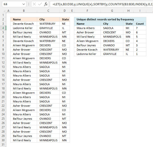
This article demonstrates how to sort records in a data set based on their count meaning the formula counts each […]
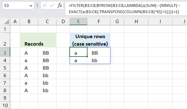
This article demonstrates two ways to extract unique and unique distinct rows from a given cell range. The first one […]
Excel categories
58 Responses to “Filter unique distinct records”
How to comment
How to add a formula to your comment
<code>Insert your formula here.</code>
Convert less than and larger than signs
Use html character entities instead of less than and larger than signs.
< becomes < and > becomes >
How to add VBA code to your comment
[vb 1="vbnet" language=","]
Put your VBA code here.
[/vb]
How to add a picture to your comment:
Upload picture to postimage.org or imgur
Paste image link to your comment.
[...] Filed in Excel on Feb.02, 2009. Email This article to a Friend In a previous article “Automatically filter unique row records from multiple columns“, i presented a solution to filter out unique values from several columns. In this article i [...]
This really is brilliant. Can I ask for one modification? How can I count the number of transactions per person?
Anura,
Formula in H8:
=SUMPRODUCT(--(E8=$A$2:$A$11)) + ENTER.
[...] We can verify the calculation by extracting all unqiue distinct records from the above table. I am using a formula from this blog article: Filter unique distinct row records in excel 2007 [...]
Oscar, this works great. Keep up the great work.
Hi Oscar,
Thank you for this sample, it is really useful.
I am trying to use it for one control sheet that I have, however I have found a problem which I am not able to fix, I hope you can help me.
The problem happens if you have an event in the current month that had already occurred in a previous month. In that case that event will not appear in the list of unique events for the current month.
For instance, in the sample you have, assuming today’s date is 5-May-2010 and if you replace the name in the first event (cell B5) with Jim Smith (instead of John Doe), the list of unique events for May 2010 will show only the event of line 7 and not the one of line 8. The event of line 8 has occurred in April and not in May, but it is still filtered and not shown in the final result.
I hope you understand my explanation and also that you can find a solution.
Thank you in advance,
MV.
MV,
You are right!
I have changed this post.
Thanks for bringing this to my attention!
Hi Oscar,
Thanks a lot!
MV
That is just awesome.
I tried equating the value "Branch A" itself in the formula instead of its address and it worked perfectly.
Thanks Oscar!
Vashi,
You are welcome!
Occar, your breakdown above worked for me, HOWEVER, i am using a date vs. Branch A. Needless to say, my spreadsheet is dynamic so i need the $F$1, in this scenario to map to a different page. When i simply change the formula to ='High Level Summary'!U3 (result = 1/10/2013 for example), my results turn to errors. It works fine as long as my date is just a date and not a formula. I even tried using INDIRECT prior to ='High Level Summary'!U3. A dropdown box is what dictates the date to be used. PLEASE HELP.... :(
Jana
Jana, can you provide the formula? Maybe your dates are not excel dates?
How excel stores dates
When I tried the workbook that was uploaded to this post-reply and pressed with left mouse button on the formula bar for cell C19 and hit 'ENTER' (without actually changing anything) and I get an #N/A record.
I'm running excel 2010, so I can only assume that the code in cell C19 'may' not work in 2010? Could this be possible? If so, can you help me with code that would work in Excel 2010??
Carlos,
When I tried the workbook that was uploaded to this post-reply and pressed with left mouse button on the formula bar for cell C19 and hit 'ENTER' (without actually changing anything) and I get an #N/A record.
That is one of the disadvantages with array formulas. If you edit an array formula (even though you don´t do any changes) you must enter it as an array formula. See: How to create an array formula, above.
I'm running excel 2010, so I can only assume that the code in cell C19 'may' not work in 2010? Could this be possible? If so, can you help me with code that would work in Excel 2010??
It works in excel 2010.
Oscar,
This is a pretty awesome solution!
I am trying to include your formula in an dashboard that shows dynamic results depending on the look-up value. I'm struggling with hiding error values (i.e. "#N/A") for the formula in the "Name" column.
I've already tried a few methods for hiding zero and error values that work with other formulas, but I can't seem to make anything work for your formula.
Can you help?
Thanks!
Dave
Looks like one way to do it is:
=IFERROR(INDEX($A$2:$C$11,MATCH(0,COUNTIF($E$7:$E7,$A$2:$A$11)+($B$2:$B$11$F$1),0),COLUMN(A1)),"")
This is a thing of beauty.
Very helpful - thank you!
dubdub,
thank you for commenting!
Thank you. This was very helpful as I wanted to extract personal data for league members (using the team as the criteria) from a league data sheet to a team data sheet.
I used David Myers' suggestion for ignoring #N/A error messages in empty rows but wonder if anyone can suggest a way to "hide" the zeros that appear when I have an incomplete row with empty cells. I assume I will need to use a nested if function in the column reference but can't get the syntax right.
I would really value any suggestions.
Thanks
Does this work if your data is on a different tab?
Tim,
Yes, change cell references.
Example,
=INDEX($A$2:$C$11, MATCH(0, COUNTIF($E$7:$E7, $A$2:$A$11)+($B$2:$B$11<>$F$1), 0), COLUMN(A1))
becomes
=INDEX(sheet2!$A$2:$C$11, MATCH(0, COUNTIF($E$7:$E7, sheet2!$A$2:$A$11)+(sheet2!$B$2:$B$11<>$F$1), 0), COLUMN(A1))
Hi ,
Is these work on the more column. i have 1400 column and this formula not working.
data is much bigger.
I am want agent project list.
i want list of project on which agent has worked.
Regards,
Krunal
Krunal,
Yes, you need a custom function (vba).
how would you add another criteria, I am looking to do this with the date and time as the criteria to match.
john dalton,
If the start date is in F1 and end date is in F2 and the dates are in cell range B2:B11:
=INDEX($A$2:$C$11, MATCH(0, COUNTIF($E$7:$E7, $A$2:$A$11)+(($B$2:$B$11>$F$1)*($B$2:$B$11<$F$2)), 0), COLUMN(A1))
How do I add another additional criteria? Say if I wanted to pull a unique list of branches and invidiuals
Justine,
perhaps this is helpful:
Filter unique distinct row records in excel 2007
Hi Oscar,
I need help as well. Suppose that i needed to find the top 20 names with the highest amounts in a Branch. I've tried with the LARGE function but i can't make it work.
Thanks
Hello,
Thanks for this! It's saved me. However, I would like to modify this formula so that it doesn't summarize by name. So using your example, I would want to see Frank's name three times, Joe's name three times, etc. I want my unique distinct list to be the same as the original list, I just want to filter out those names that aren't Branch A.
Thanks.
Chuck
Array formula in cell E8:
=INDEX($A$2:$C$11, SMALL(IF($F$1<>$B$2:$B$11, MATCH(ROW($B$2:$B$11), ROW($B$2:$B$11)), ""), ROW(A1)), COLUMNS($A$1:A1))
Thanks, Oscar! Works like a champ. However, I would like to point out that this formula only works if your original table starts in A1. So the last part of your formula:
...ROW(A1)), COLUMNS($A$1:A1))
I had to come up with another way to get the correct values here. Once I did it worked great. Thank you.
Hi Oscar,
This works as a charm, however (as in previous comment) I need value be displayed all times it appears in the list. Is there any way to tell this formula not to ignore repetitive values?
I mean the result should look like
Frank Branch A
Frank Branch A
Frank Branch A
Joe Branch A
Mike Branch A
Joe Branch A
Joe Branch A
Thanks in advance!
I don't have any questions. I just want to say that you are awesome.
Thanks for your helpful and clear examples. Following your same example – how about if from a long list of branches, I need to extract the amounts of sub-set of branches. For examples, need the amounts from 7 out of 20 branches, just to illustrate an example. How do I name the string of non-consecutive branch numbers? Thanks again
Thanks for your helpful and clear examples. Following your same example – how about if from a long list of branches, I need to extract the amounts of sub-set of branches. For examples, need the amounts from 7 out of 20 branches, just to illustrate an example. How do I specify a string of non-consecutive branch numbers?
Sorry for the multiple entries, something is wrong on this end
Hi Oscar,
I dint understand how this countif is working. I can see that the range is smaller than the criteria. Can you please explain the logic through the first principles.
Thanks.
Hi Chuck
How can I sort my data while fetching. Lets say, I want my data to be sorted ascending order wise depending on amount. I don't want a help column. How can I do it in one go, while I am pulling the data using your formula
I have what I think is a very simple process I want to do, but I cannot find the answer on the internet because I do not know what to call it in 'excel speak'. I have a list of students and their reading level (numerical). I just want it to dynamically create lists of all the students in each level.
e.g.
Students Level
studentA 2
studentB 9
studentC 7
studentD 3
studentE 9
etc (in two columns) and I want to then create a table with the levels as the headings and the students names to automatically go under the level.
e.g.
1 2 3... ...9
studentA studentB
student E
How can I do this?
Hi Oscar,
I'm starting to learn Excel now. And I have a spreadsheet similar to a data entry. My job is to go through weekly data to see which kid is in trouble. My question is, Is there a formula I can set where it list down data from a certain range. For example if I want to view data from the 5/18/2016 to 5/24/2016.
Thanks
John
I recommend you convert your data table to an excel defined table and apply a date filter to your date column.
https://support.office.com/en-us/article/Overview-of-Excel-tables-7ab0bb7d-3a9e-4b56-a3c9-6c94334e492c
Hi there,
I have a dataset and I wish to show, in a separate tab, a distinct list based on two criterion. What would I need to do?
Thanks, Kevin
Kevin,
This formula has one criterion (bolded):
=INDEX($A$2:$C$11, MATCH(0, COUNTIF($E$7:$E7, $A$2:$A$11)+($B$2:$B$11<>$F$1), 0), COLUMN(A1))
If you need two criteria, see this formula:
=INDEX($A$2:$C$11, MATCH(0, COUNTIF($E$7:$E7, $A$2:$A$11)+($B$2:$B$11<>$F$1)*($A$2:$A$11<>"Frank"), 0), COLUMN(A1))
It looks for a criterion in column A and another criterion in column B.
This formula looks for two criteria ($F$1:$F$2) in cell range $B$2:$B$11:
=INDEX($A$2:$C$11, MATCH(0, COUNTIF($E$7:$E7, $A$2:$A$11)+COUNTIF($F$1:$F$2,"<>"&$B$2:$B$11), 0), COLUMN(A1))
Hi Oscar,
I'm using a very similar formula to yours:
=IFERROR(INDEX(all_names, MATCH(0, IF($D$2=all_groups, COUNTIF(D$4:D4, all_names), ""), 0)),"")
This works well. However, if I try to change it to include an OR function it no longer work:
=IFERROR(INDEX(all_names, MATCH(0, IF(OR($D$2=all_groups,$D$2=all_groups_2,$D$2=all_groups_3), COUNTIF(D$4:D4, all_names), ""), 0)),"")
Any idea what I'm doing wrong?
Thanks,
Jake
Jake,
Try this:
=IFERROR(INDEX(all_names, MATCH(0, IF(($D$2=all_groups)+($D$2=all_groups_2)+($D$2=all_groups_3), COUNTIF(D$4:D4, all_names), ""), 0)),"")
Hello Oscar,
What code is needed to cause cells in Columns F - I to fill with the contents of Columns C - E when a cell in Column B includes a numeric value?
Liam,
See this post:
https://www.get-digital-help.com/filter-rows-where-a-cell-contains-a-numeric-value/
THANK YOU SO MUCH.... IT IS VERY VERY VERY HELPFUL AND I AM TOO MUCH EXCITING TO LEARN THIS FORMULA..... I WOULD LIKE TO SAY AGAIN *"THANK YOU SO MUCH...."*
Oscar,
I have a similar issue and would ask if you can help with the final step of extracting a list of names from a 'helper' column that fall within a date range?
I have a worksheet with 2 tabs, one for DATA (over 4,000 rows) and the other is used to do lookups and reflect calculations on the data (REPORT). I attach an image of a spreadsheet I created just to give you an idea of what the columns and ranges are: https://postimg.org/image/c203uwp5h/
On the DATA tab, there are 2 columns of data 'Dates' and 'Agent' (these are the range names as well) - and I've created a 3rd column using INDEX/MATCH that contains a unique list of agent names found in the 'AGENT' range (named range of AGENTLIST).
Now I need to use this 'helper' column to derive a 2nd list (on the REPORT Tab) of just those agent names that have records that fall within two dates (date fields also on the REPORT Tab). As I change the dates, I would expect the 2nd list of names to be updated as the sheet recalculates.
If I had my 'druthers', it would be GREAT if that list is sorted.
I do not have the excel experience to do this, and I derived the first 'unique' list only after much studying of all the similar posts on this site (great site BTW). I hope you can help me.
Thanks,
Rich
Rich Darlington
Use a pivot table!
https://www.get-digital-help.com/excel-pivot-tables/
Dear
How can I make this work by having the names F5:F7 alphabetically with 2 conditions ?
Thanks
Oliver
Hi,
Great site!
I need help comparing two ranges and extracting unique names on one side, and repeated names on the other.
For instance, in one range I have a list of all the employees currently working in my office. They are in a separate sheet named "operadores".
They don't have to come to work every day, so in a different sheet on my workbook, I have a grid that lists the days of the semester in column C (there's a blank row between each day), and somewhere in those two rows there's the name of the employees that are assigned to work that day, next to the assignment they are working on.
I would need a formula that looks what the names of my employees are, and checks whether they are assigned that day.
After that, I would split it in two:
- On one side I would need to know who is free to be assigned to a different project.
- On the other side, I would need to know who is assigned so I can call them and let them know they have to come to work.
Is that possible? I'm working on Excel 2013.
Thanks!
Alejandra
Alejandra
Can you describe in greater detail how data is arranged on your worksheets? Perhaps an example or a picture?
[…] Extract a unique distinct list and sum amounts based on a condition […]
Thanks for posting this example. It has been so helpful.
Question: How would I do the same thing if I only want to copy the unique events from two non-adjacent columns, for example, column A and D, and not copy columns B and C?
Thank you
Shaun
I have a table with four columns Month, Brand Name, Executive Name, and Shop Name.
I am trying to find out, how many shop can sale executive wise month wise brand wise. I am trying count shop name but not get success.
Hope you are able to help. Thanks in advance.
Month Shop Name Executive Name Brand Name
Jan.20 Shiv Shakti & Sons Hari Mohan Red Pen
Jan.20 Body Shop Rajesh Singh Blue Pen
Jan.20 Stop & Shop Govind Ram Green Pen
Feb.20 Shiv Shakti & Sons Hari Mohan Blue Pen
Feb.20 Body Shop Rajesh Singh Green Pen
March.20 Shiv Shakti & Sons Hari Mohan Red Pen
March.20 Body Shop Rajesh Singh Blue Pen
March.20 Stop & Shop Govind Ram Green Pen
March.20 Shop Clue Jai Prakesh Red Pen
Oscar,
I have a list with duplicate values in 2 columns. How do I extract one distinct list with two columns. They are not two separate lists. They are columns with two different column headings: Type & Letter
Type Letter
Car A
Bike D
Car A
Bike D
Bike E
Result:
Car A
Bike D
Bike E
Car A
I made a mistake. The result should be
Type Letter
Car A
Bike D
Bike E