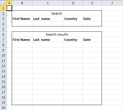
Lookup with any number of criteria

This article demonstrates a formula that allows you to search a data set using any number of conditions, however, one condition per column. The search functionality matches the entire value in a cell, no wildcard matches.
It also demonstrates how to extract the records using the Advanced Filter. The Advanced Filter is a built-in Excel feature that allows you to do more complicated filtering than the regular Filter feature or an Excel Table can accomplish.
What's on this page
- Lookup with an unknown number of criteria - Array Formula
- Lookup with an unknown number of criteria - Advanced Filter
- Excel Table and slicers
- How to filter using OR logic between columns - Advanced Filter
- Find entry based on conditions
- Lookup multiple values in one cell - UDF
- Lookup multiple values in one cell - Excel 365
1. Lookup with an unknown number of criteria - Array Formula
Rashid asks:I used your array formula with great success to find the search results from multiple criteria. However, my problem is modifying your formula. In the above example you have shown us, you have two criteria. And you distinguish the two criteria by using *.
My question is: what would you do if you don't know the predetermined number of criteria. So let's say the person searching only specifies security and not date. Or only date, and not security. Or maybe both. The problem is you don't know from beforehand.
How would you go about solving this problem?
Your help is greatly appreciated, thanks so much!!
The animated image above shows different conditions being used and how the formula instantly returns records that match. It also shows that you can use multiple conditions to narrow down the results. The data is located on worksheet Sheet2.
Formula in cell B8:
This formula requires you to enter it as an array formula if you have an older Excel version than an Excel 365 subscription, the steps to enter an array formula are below.
This formula does not spill values automatically if needed, you have to type the formula in a cell and then press enter. Copy the cell and paste to adjacent cells below and to the right as far as needed.
How to enter an array formula
- Select cell B8
- Type the above array formula
- Press and hold CTRL + SHIFT
- Press Enter
- Release all keys
If you got it right, there is now a { before the array formula and a } after the array formula.
How to copy array formula
- Copy cell B8
- Paste to C8:E8
- Copy cell range B8:E8
- Paste to cell range B9:E19
Explaining the array formula in cell B8

The image above shows the data on worksheet Sheet2, it contains random names, countries and dates.
I recommend the "Evaluate Formula" feature if you want to see the formula calculations in greater detail.

- Select the cell containing the formula you want to learn.
- Go to tab "Formulas" on the ribbon.
- Press with left mouse button on the "Evaluate Formula" button. A dialog box appears.
- Press with left mouse button on the "Evaluate" button to move to next calculation step.
- Press with left mouse button on "Close" to dismiss the dialog box.
Step 1 - Count the number of cells in each table column that meet the criteria and add the arrays
The COUNTIF function counts values based on a condition or criteria. There are four COUNTIF functions, as many as there are columns in the data set.
The returning arrays are added together, this means we apply OR logic to the result meaning if any of the values in the same position are one the result is one or more.
COUNTIF($B$4, Sheet2!$A$2:$A$21)+COUNTIF(Sheet1!$C$4, Sheet2!$B$2:$B$21)+COUNTIF(Sheet1!$D$4, Sheet2!$C$2:$C$21)+COUNTIF(Sheet1!$E$4, Sheet2!$D$2:$D$21)
becomes
{0;0;1;0;0;0;0;0;0;0;0;0;0;0;0;0;0;0;0;0})+{0;0;0;0;0;0;0;0;0;0;0;0;0;0;0;0;0;0;0;0}+{0;0;0;0;0;0;0;0;0;0;0;0;0;0;0;0;0;0;0;0}+{0;0;1;0;0;0;0;0;0;0;0;0;0;0;1;0;0;0;0;0}
and returns
{0;0;2;0;0;0;0;0;0;0;0;0;0;0;1;0;0;0;0;0}
This means that row 3 (relative row) matches two conditions. Why is that? 2 is the third value in the array.
Step 2 - Count the number of criteria matching and compare with each value in the array above
The IF function has three arguments, the first one must be a logical expression. If the expression evaluates to TRUE then one thing happens (argument 2) and if FALSE another thing happens (argument 3).
IF(COUNTA($B$4:$E$4)=(COUNTIF($B$4, Sheet2!$A$2:$A$21)+COUNTIF(Sheet1!$C$4, Sheet2!$B$2:$B$21)+COUNTIF(Sheet1!$D$4, Sheet2!$C$2:$C$21)+COUNTIF(Sheet1!$E$4, Sheet2!$D$2:$D$21)), MATCH(ROW(Sheet2!$D$2:$D$21), ROW(Sheet2!$D$2:$D$21)), "")
becomes
IF(2={0;0;2;0;0;0;0;0;0;0;0;0;0;0;1;0;0;0;0;0}, MATCH(ROW(Sheet2!$D$2:$D$21), ROW(Sheet2!$D$2:$D$21)), "")
becomes
IF(2={0;0;2;0;0;0;0;0;0;0;0;0;0;0;1;0;0;0;0;0}, {1;2;3;4;5;6;7;8;9;10;11;12;13;14;15;16;17;18;19;20}, "")
becomes
IF({FALSE; FALSE; TRUE; FALSE; FALSE; FALSE; FALSE; FALSE; FALSE; FALSE; FALSE; FALSE; FALSE; FALSE; FALSE; FALSE; FALSE; FALSE; FALSE; FALSE}, {1;2;3;4;5; 6;7;8;9;10; 11;12;13;14; 15;16;17;18;19;20}, "")
and returns
{"";"";3;""; "";"";"";"";""; "";"";"";"";"";""; "";"";"";"";""}
Step 3 - Find the k-th smallest row number
To be able to return a new value in a cell each I use the SMALL function to filter column numbers from smallest to largest.
SMALL(IF(COUNTA($B$4:$E$4)=(COUNTIF($B$4, Sheet2!$A$2:$A$21)+COUNTIF(Sheet1!$C$4, Sheet2!$B$2:$B$21)+COUNTIF(Sheet1!$D$4, Sheet2!$C$2:$C$21)+COUNTIF(Sheet1!$E$4, Sheet2!$D$2:$D$21)), MATCH(ROW(Sheet2!$D$2:$D$21), ROW(Sheet2!$D$2:$D$21)), ""), ROW(A1))
becomes
SMALL({"";"";3;""; "";"";"";"";""; "";"";"";"";"";""; "";"";"";"";""}, ROW(A1))
and returns 3.
Step 4 - Return corresponding value from data table on sheet 2
The INDEX function returns a value based on a cell reference and column/row numbers.
INDEX(Sheet2!$A$2:$D$21, SMALL(IF(COUNTA($B$4:$E$4)=(COUNTIF($B$4, Sheet2!$A$2:$A$21)+COUNTIF(Sheet1!$C$4, Sheet2!$B$2:$B$21)+COUNTIF(Sheet1!$D$4, Sheet2!$C$2:$C$21)+COUNTIF(Sheet1!$E$4, Sheet2!$D$2:$D$21)), MATCH(ROW(Sheet2!$D$2:$D$21), ROW(Sheet2!$D$2:$D$21)), ""), ROW(A1)), COLUMN(A1))
becomes
INDEX(Sheet2!$A$2:$D$21, 3, COLUMN(A1))
becomes
INDEX(Sheet2!$A$2:$D$21, 3, 1)
and returns Keisha.
Step 5 - Check if there are more than 0 (zero) citeria
The COUNTA function counts the non-empty or blank cells in a cell range.
COUNTA($B$4:$E$4)<>0
becomes
2<>0
and returns TRUE
Step 6 - Return value if there are more than zero criteria
IF(COUNTA($B$4:$E$4)<>0, INDEX(Sheet2!$A$2:$D$21, SMALL(IF(COUNTA($B$4:$E$4)=(COUNTIF($B$4, Sheet2!$A$2:$A$21)+COUNTIF(Sheet1!$C$4, Sheet2!$B$2:$B$21)+COUNTIF(Sheet1!$D$4, Sheet2!$C$2:$C$21)+COUNTIF(Sheet1!$E$4, Sheet2!$D$2:$D$21)), MATCH(ROW(Sheet2!$D$2:$D$21), ROW(Sheet2!$D$2:$D$21)), ""), ROW(A1)), COLUMN(A1)), "")
becomes
IF(TRUE, "Keisha", "")
and returns "Keisha" in cell B8.
2. Lookup with an unknown number of criteria [Advanced Filter]

The image above shows the filtered data in-place using a condition on row 3. It uses Excel's built-in feature named Advanced Filter.
There are no formulas in this example. I made room for conditions above the data list. I copied the header names to a row above the data.
Here is how to set it up.
- Go to tab "Data" on the ribbon.
- Press with left mouse button on the "Advanced" button. A dialog box appears.

- You can filter the list in-place or copy to another location. I chose to filter in-place.
- The list range lets you select the data you want to filter.
Note, select the column header names as well.
- Select your criteria in "The Criteria range:". Don't forget to include your column header names.
- Press with left mouse button on OK button.

The image above shows the filtered list, the colored row numbers indicate that the list is filtered. Press with left mouse button on the "Clear" button on the ribbon to delete the filter, all data will be visible again.
I recommend you check out the Advanced Filter category if this feature is interesting for you.
3. Excel Table and slicers

The image above shows the data set converted to an Excel Table and four slicers above the Excel Table. Slicers were introduced in Excel version 2010.
They allow you to quickly filter data by press with left mouse button oning on values in the slicer. You can only use slicers with Excel Tables and Pivot Tables, however, both Excel Tables and Slicers are really easy to create. Let us begin creating an Excel Table.
How to convert a data set to an Excel Table

- Select any cell in the data set.
- Press CTRL + T to open the "Create Table" dialog box. See image above.
- Enable checkbox "My Table has headers" if true.
- Press with left mouse button on OK button.
How to create Slicers

- Select any cell in the Excel Table. A new tab named "Table Design" appears on the ribbon.
- Go to tab "Table Design" on the ribbon.
- Press with left mouse button on "Insert Slicers" button. A dialog box appears, see image above. Press with left mouse button on checkboxes to insert a slice for each, the names next to checkboxes are column header names.
- Press with left mouse button on OK button.
- Excel inserts a slicer for each selected checkbox.

- Move and resize each slicer.
How to select, move and resize slicers

Press with left mouse button on with left mouse button on a slicer you want to select. A selected slicer shows sizing handles. They are white circles that appear on each corner and side.

Press and hold CTRL key and then press with left mouse button on multiple slicers to select them. Selected slicers have sizing handles visible.
To move a slicing handle press and hold on a selected slicer and then drag with mouse to a new location. Release left mouse button to let go.
To resize a slicers press and hold on any sizing handle, then drag with mouse to resize.
Recommended articles
- Use slicers to filter data (Microsoft)
- Filter by using advanced criteria (Microsoft)
4. How to filter using OR logic between columns - Advanced Filter
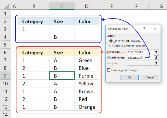
4.1. How to filter using OR logic between columns
The built-in filter feature in Excel is a powerful tool, however, it won't allow you to filter with OR logic between columns.
This is where the Advanced Filter comes into the picture. It lets you do that and I will show you how now.
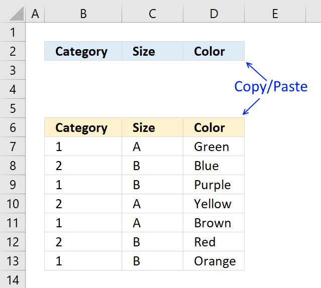
Copy your table headers and paste them somewhere on your worksheet.
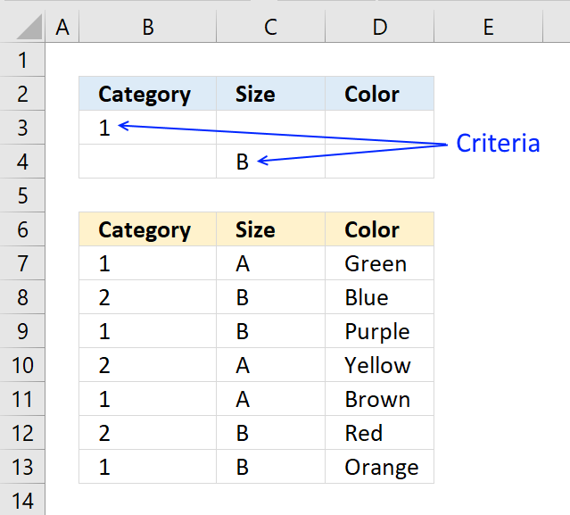
Type the criteria you want to use right below the new headers, each below the header you want to filter, see picture below.
Make sure the condition is the only one on each row.
Now it is time to start the Advanced Filter. Go to tab "Data" on the ribbon and press with left mouse button on "Advanced Filter" button.

The "Advanced Filter" settings window appears.
Press with mouse on "List range:" field and select cell range B6:D13 (your data you want to filter).
Press with mouse on "Criteria range:" field and select cell range B2:D4 (your criteria you want to use).
Press with left mouse button on OK button.
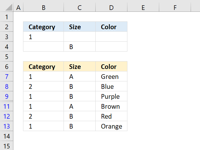
The blue rows to the left show you that you have applied a filter to your data.
To clear the filter simply press with left mouse button on the clear button on the ribbon tab "Data".
![]()
Get Excel *.xlsx file
How to filter with OR logic between columns.xlsx
4.2. Advanced custom date filter
Question: How do I filter the last xx years or xx months in Excel?
How do I exclude the current month when using the year to date filter in Excel?
Answer: Use advanced filter with criteria ranges. I have calculated the exact dates needed to create the criteria ranges.
I will go through the exact steps on how to accomplish the date filter.
The picture below shows the calculation of the dates, the criteria ranges and the list to filter.

How to create a criteria range
- Copy the header of the list to a new location, see cell A16:C16 in the above picture.
- Type the criteria, see A17:B17 in the above picture.
- Formula in A17:
="<=2009-07-31" + ENTER
Formula in B17:
=">=2009-01-01" + ENTER
How to filter a list using a criteria range
- Press with left mouse button on "Data" in the ribbon
- Press with left mouse button on Advanced

- Select List range: A27:C64

- Select the criteria range A16:C17
- Press with left mouse button on OK!
The new filtered list.

Repeat the above steps to filter the last xx years or xx months using the criteria ranges.
Get excel example file.
filter-a-list-of-dates.xlsx
(Excel 2007 Workbook *.xlsx)
5. Find entry based on conditions
![]()
Hello Oscar,
I am building a spreadsheet for tracking calls for my local fire department. I have a column "a" as an incident number. the incident number is a one-time yearly number usage.
Column "c" is apparatus name and there are 1 of 8 possible names may be used in this cell. column "h" has the formula to give me the time spent on the scene.
I am needing help getting sheet 2 to tag the time spent on a call per apparatus. Sheet 2 is the names of personnel on the scene. I want to put the time on scene according to what apparatus they were on for each incident.
example:
column "a" newest entry is #10
column "c" is "bt1" or "bt2" or "e1" or "e3" or "e4" or "e5" or "pov" or "stby"
There often will be multiple rows with the same incident# in column "a" but different apparatus in column "c".
Column "h" will have on scene time calculated by "=f5-d5"(for that row)
I need to tag on the scene time from sheet 1 column "h" to the corresponding incident number column "a" according to the apparatus column "c".
Last Total
Enroute Arrival Clear Response Incident
Incident # Date Apparatus Time Time Time Time Time
1 03/01/12 bt2 8:18 8:27 18:45 0:09:00 10:27:00
2 03/25/12 bt2 8:20 8:23 17:45 0:03:00 9:25:00
e1 17:05 17:10 17:45 0:05:00 0:40:00
e3 12:33 12:38 17:45 0:05:00 5:12:00
3 03/26/12 e4 7:45 8:08 10:22 0:23:00 2:37:00
4 03/26/12 bt2 11:14 11:16 11:29 0:02:00 0:15:00
5 03/27/12 pov 13:10 13:20 18:36 0:10:00 5:26:00
stby 13:15 13:20 18:36 0:05:00 5:21:00
bt1 13:15 13:20 18:36 0:05:00 5:21:00
bt2 13:16 13:21 18:36 0:05:00 5:20:00
6 03/28/12 e1 8:18 8:27 18:45 0:09:00 10:27:00
e3 8:20 8:30 18:45 0:10:00 10:25:00
7 03/28/12 bt1 8:20 8:23 17:45 0:03:00 9:25:00
e5 9:00 9:03 17:45 0:03:00 8:45:00
8 03/28/12 bt2 9:20 9:22 9:59 0:02:00 0:39:00
9 03/29/12 e1 17:45 17:50 18:00 0:05:00 0:15:00
The array formula reads incident numbers and apparatus values, therefore, I entered missing incident numbers.
How to enter a formula in blank cells
- Select cell range A1:A17
- Press F5
- Press with left mouse button on "Special"
- Press with left mouse button on "Blanks"
- Press with left mouse button on "OK"
- Type =A3
- Press and hold Ctrl
- Press Enter
Array formula in sheet2
![]()
Array formula in cell C2:
How to enter an array formula
- Double press with left mouse button on cell C2
- Copy/Paste array formula
- Press and hold Ctrl and Shift
- Press Enter
How to copy array formula
- Select cell C2
- Copy (Ctrl + c)
- Select cell range C3:C10
- Paste (Ctrl + v)
Explaining array formula in cell C2
Step 1 - Find incident number and Apparatus value
(B2=Sheet1!$C$2:$C$17)*(A2=Sheet1!$A$2:$A$17)
becomes
("bt2"={"bt2";"bt2";"e1";"e3";"e4";"bt2";"pov";"stby";"bt1";"bt2";"e1";"e3";"bt1";"e5";"bt2";"e1"} ) * (1={1;2;2;2;3;4;5;5;5;5;6;6;7;7;8;9})
becomes
{1;0;0;0;0;0;0;0;0;0;0;0;0;0;0;0}
Step 2 - Convert array to row numbers
IF((B2=Sheet1!$C$2:$C$17)*(A2=Sheet1!$A$2:$A$17), MATCH(ROW(Sheet1!$A$2:$A$17), ROW(Sheet1!$A$2:$A$17)), "")
becomes
IF({1;0;0;0;0;0;0;0;0;0;0;0;0;0;0;0}, MATCH(ROW(Sheet1!$A$2:$A$17), ROW(Sheet1!$A$2:$A$17)), "")
becomes
IF({1;0;0;0;0;0;0;0;0;0;0;0;0;0;0;0}, {1;2;3;4;5;6;7;8;9;10;11;12;13;14;15;16;17}, "")
and returns
{1;"";"";"";"";"";"";"";"";"";"";"";"";"";"";""}
Step 3 - Find smallest value in array
MIN(IF((B2=Sheet1!$C$2:$C$17)*(A2=Sheet1!$A$2:$A$17), MATCH(ROW(Sheet1!$A$2:$A$17), ROW(Sheet1!$A$2:$A$17)), ""))
becomes
MIN({1;"";"";"";"";"";"";"";"";"";"";"";"";"";"";""})
and returns
1
Step 4 - Return an error if no value is found
IF(SUM(--(B2=Sheet1!$C$2:$C$17)*(A2=Sheet1!$A$2:$A$17))=0, NA(), MIN(IF((B2=Sheet1!$C$2:$C$17)*(A2=Sheet1!$A$2:$A$17), MATCH(ROW(Sheet1!$A$2:$A$17), ROW(Sheet1!$A$2:$A$17)), "")))
becomes
IF(SUM(--(B2=Sheet1!$C$2:$C$17)*(A2=Sheet1!$A$2:$A$17))=0, NA(), 1))
becomes
IF(SUM({1;0;0;0;0;0;0;0;0;0;0;0;0;0;0;0})=0, NA(), 1))
becomes
IF(1=0, NA(), 1))
becomes
IF(False, NA(), 1))
and returns 1
Step 5 - Return time value
=INDEX(Sheet1!$H$2:$H$17, IF(SUM(--(B2=Sheet1!$C$2:$C$17)*(A2=Sheet1!$A$2:$A$17))=0, NA(), MIN(IF((B2=Sheet1!$C$2:$C$17)*(A2=Sheet1!$A$2:$A$17), MATCH(ROW(Sheet1!$A$2:$A$17), ROW(Sheet1!$A$2:$A$17)), ""))))
becomes
=INDEX(Sheet1!$H$2:$H$17, 1)
becomes
=INDEX({0,435416666666667; 0,392361111111111; 0,0277777777777778; 0,216666666666667; 0,109027777777778; 0,0104166666666667; 0,226388888888889; 0,222916666666667; 0,222916666666667; 0,222222222222222; 0,435416666666667; 0,434027777777778; 0,392361111111111; 0,364583333333333; 0,0270833333333333; 0,0104166666666667}, 1)
and returns 0,435416666666667 in cell C2. Formatted as time, 10:27:00
6. Lookup multiple values in one cell - UDF
A UDF (User defined Function) is an Excel function that you can build yourself which is great if you can't find a prebuilt one that suits your needs.
You create a UDF the same way you create a macro using VBA code in the VB Editor (Visual Basic Editor), VBA stands for Visual Basic for Applications.
I will explain in greater detail the code I used, where to put it, and how to save your workbook, later in this article.
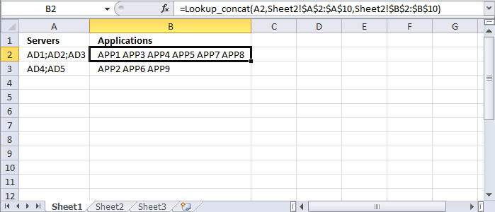
Hi Oscar
This is a very interesting function and helped me a lot so far. My file though is a bit more complicated.
I have multiple info in one cell separated with ";" (example AD1; AD2; AD3) let's say that these are servers (File name SERVERS) and in each server, I have multiple applications.
I have now another file that has all the applications per server per line in excel (each line has one server one application. Filename: APPS).
I want to start from the file SERVERS to look up the servers that are in one cell find them in the second file APPS and bring all the applications also in one cell in the file SERVERS.
Any ideas here?
Thanks in advance
C
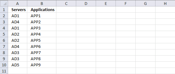
Worksheet Sheet2 contains the items and the corresponding applications.
Worksheet Sheet1 contains the concatenated items in column A and a formula in column B. The first argument in the UDF is the cell that contains the concatenated values, this cell reference is relative meaning it changes when you copy cell B2 and paste it to cells below.
The second argument is the lookup range and the third argument is the return range, both these arguments have absolute cell references.
Lookup_concat(Search_string, Search_in_col , Return_val_col )
Formula in cell B2:
VBA code
'Name the UDF and declare arguments and data types
Function Lookup_concat(Search_string As String, _
  Search_in_col As Range, Return_val_col As Range)

'Dimension variables and declare data types
Dim i As Long, result As String
Dim Search_strings, Value As Variant

'Split string using a delimiting character and return an array of values
Search_strings = Split(Search_string, ";")

'Iterate through values in array
For Each Value In Search_strings

    'Iterate through from 1 to the number of cells in Search_in_col
    For i = 1 To Search_in_col.Count

      'Check if cell value is equal to value in variable Value
      If Search_in_col.Cells(i, 1) = Value Then

        'Save the corresponding return value to variable result
        result = result & " " & Return_val_col.Cells(i, 1).Value
      End If

    'Continue with next number
    Next i

'Continue with next value
Next Value

'Return values saved to result to worksheet
Lookup_concat = Trim(result)
End Function
Where to put the code?
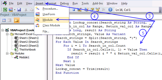
You can use the code (see instructions below) in your workbook or get the example file.
- Copy VBA code above.
- Open VB Editor (Alt+F11) and select your workbook in the Project Explorer.
- Press with left mouse button on Insert on the menu.
- Press with left mouse button on Module to create a module.
- Paste code to module1
- Exit VB Editor
7. Lookup multiple values in one cell - Excel 365

This Excel 365 formula splits a given cell value based on a specific delimiter and performs a lookup for each substring, then the corresponding value on the same row is returned and concatenated together with the remaining results.
Excel 365 formula in cell C3:
Explaining formula
Step 1 - Split cell value
The TEXTSPLIT function splits a string into an array based on delimiting values.
Function syntax: TEXTSPLIT(Input_Text, col_delimiter, [row_delimiter], [Ignore_Empty])
TEXTSPLIT(B3, ";")
becomes
TEXTSPLIT("AD1;AD2;AD3", ";")
and returns
{"AD1", "AD2", "AD3"}.
Step 2 - Compare substrings to a lookup table
The equal sign lets you compare value to value, you can also compare array to array as long as the first array is horizontal and the second array is vertical or vice versa.
TEXTSPLIT(B3, ";")=$E$3:$E$11
becomes
{"AD1", "AD2", "AD3"}={"AD1";"AD4";"AD1";"AD2";"AD2";"AD4";"AD3";"AD3";"AD5"}
and returns
{TRUE,FALSE,FALSE ; FALSE,FALSE,FALSE ; TRUE,FALSE,FALSE ; FALSE,TRUE,FALSE ; FALSE,TRUE,FALSE ; FALSE,FALSE,FALSE ; FALSE,FALSE,TRUE ; FALSE,FALSE,TRUE ; FALSE,FALSE,FALSE}
Step 3 - Convert boolean values
Step 2 returned an array of boolean values, the MMULT function can't handle boolean values. The asterisk character lets you multiply values in an Excel formula, it is also possible to multiply boolean values and in the process create their numerical equivalents.
TRUE equals 1 and FALSE equals 0 (zero).
(TEXTSPLIT(B3, ";")=$E$3:$E$11)*1
becomes
{TRUE,FALSE,FALSE ; FALSE,FALSE,FALSE ; TRUE,FALSE,FALSE ; FALSE,TRUE,FALSE ; FALSE,TRUE,FALSE ; FALSE,FALSE,FALSE ; FALSE,FALSE,TRUE ; FALSE,FALSE,TRUE ; FALSE,FALSE,FALSE}*1
and returns
{1,0,0 ; 0,0,0 ; 1,0,0 ; 0,1,0 ; 0,1,0 ; 0,0,0 ; 0,0,1 ; 0,0,1 ; 0,0,0}.
Step 4 - Create an array
We need an array of numbers that match the number of substrings found in the cell, they all need to be 1 so the MMULT function can calculate properly.
The ISTEXT function returns TRUE if argument is text.
Function syntax: ISTEXT(value)
ISTEXT(TEXTSPLIT(B3,,";"))
becomes
ISTEXT({"AD1"; "AD2"; "AD3"})
and returns
{TRUE; TRUE; TRUE}.
Step 5 - Convert boolean values
The power of character ^ lets you convert the boolean value to 1 if you calculate the power of 0 (zero).
ISTEXT(TEXTSPLIT(B3, , ";"))^0
becomes
{TRUE; TRUE; TRUE}^0
and returns {1; 1; 1}.
Step 6 - Sum numbers row-wise
The MMULT function calculates the matrix product of two arrays, an array as the same number of rows as array1 and columns as array2.
Function syntax: MMULT(array1, array2)
MMULT((TEXTSPLIT(B3, ";")=$E$3:$E$11)*1, ISTEXT(TEXTSPLIT(B3, , ";"))^0)
becomes
MMULT({1,0,0 ; 0,0,0 ; 1,0,0 ; 0,1,0 ; 0,1,0 ; 0,0,0 ; 0,0,1 ; 0,0,1 ; 0,0,0},{1; 1; 1})
and returns
{1; 0; 1; 1; 1; 0; 1; 1; 0}.
Step 7 - Filter values based on array
The FILTER function extracts values/rows based on a condition or criteria.
Function syntax: FILTER(array, include, [if_empty])
FILTER($F$3:$F$11, MMULT((TEXTSPLIT(B3, ";")=$E$3:$E$11)*1, ISTEXT(TEXTSPLIT(B3, , ";"))^0))
becomes
FILTER({"APP1";"APP2";"APP3";"APP4";"APP5";"APP6";"APP7";"APP8";"APP9"}, {1; 0; 1; 1; 1; 0; 1; 1; 0})
and returns
{"APP1"; "APP3"; "APP4"; "APP5"; "APP7"; "APP8"}.
Step 8 - Concatenate values
The TEXTJOIN function combines text strings from multiple cell ranges.
Function syntax: TEXTJOIN(delimiter, ignore_empty, text1, [text2], ...)
TEXTJOIN(" ", TRUE, FILTER($F$3:$F$11, MMULT((TEXTSPLIT(B3, ";")=$E$3:$E$11)*1, ISTEXT(TEXTSPLIT(B3, , ";"))^0)))
becomes
TEXTJOIN(" ", TRUE, {"APP1"; "APP3"; "APP4"; "APP5"; "APP7"; "APP8"})
and returns
"APP1 APP3 APP4 APP5 APP7 APP8".
Advanced filter excel category

First, let me explain the difference between unique values and unique distinct values, it is important you know the difference […]
Lookups category
Table of Contents How to perform a two-dimensional lookup Reverse two-way lookups in a cross reference table [Excel 2016] Reverse […]
Excel categories
15 Responses to “Lookup with any number of criteria”
Leave a Reply
How to comment
How to add a formula to your comment
<code>Insert your formula here.</code>
Convert less than and larger than signs
Use html character entities instead of less than and larger than signs.
< becomes < and > becomes >
How to add VBA code to your comment
[vb 1="vbnet" language=","]
Put your VBA code here.
[/vb]
How to add a picture to your comment:
Upload picture to postimage.org or imgur
Paste image link to your comment.
The advanced filter works perfectly with the dates intervals >DD/MM/YY and DD/MM/YY; however when you record it under a MACRO it does not work !!!
Can someone help?
The advanced filter works perfectly with the dates intervals >DD/MM/YY and <DD/MM/YY; however when you record it under a MACRO it does not work !!!
Can someone help?
What did you record in your macro?
Hi Oscar,
This is great and compliments your Multiple Criteria and Multiple Matches series of posts very well. However I have been trying to modify the array formulas in the 3rd and 4th posts of that series to cope with wildcard searches or part cell matches and thought this post may help but not so far unfortunately.
I have tried numerous approaches but can't seem to get a multiple criteria series of "searches" (or counts) to work with anything but exact data.
I'm trying to search for part of a serial number e.g.(A110 within a string A110E12694369020 as one of my search inputs. In this case it is always the first 4 digits but I'd like to be able to input just A1 or *A1* into a search cell and not rely on reviewing the first 4 characters as this is not always the result for these serial numbers.
I'm also looking for items with corresponding dates equal or before a certain due date search string - your 4th post to Lookup-with-multiple-criteria-and-display-multiple-search-results-using-excel-formula-part-4-john helped me resolve this criteria though.
Finally I'm trying another 'wildcard' search and to find FSS (or *FSS*) OR the exact inverse of this - so NOT containing FSS (or *FSS*) - and both of these search criteria are proving elusive to me.
All the data I have is in a large table but I'm not sure if I can alter it to be an Excel Table (which might help), as it is in a sheet that is deleted and replaced by an irregular macro from another workbook and this may corrupt a Table setup(?). It can not be a Pivot as the data is in a shared workbook and Pivot Tables do not update when in shared documents - hence the Array solution I am trying to develop. I have successfully named the columns of ranges I need though without loosing them on an update of data.
To summarise - I'd like to search by some form of wildcard; *app* to return a positive result for "apple" and to search for the opposite; have a criteria that would exclude "apple" using soemthing like *app*
Although I have around 80 columns I'm just looking to return the serial number in say Column A based on these multiple criteria; Col B <= a date, Col C does NOT contain a wildcard string *whatever*, Col D DOES contain a different wildcard string, Col E EXACTLY equals a third search string etc. I am happy to build up the criteria to more columns beyond this if I can resolve the NOT and the wildcard elements.
I'd really appreciate some further pointers, thanks Oscar!
[…] was inspired by this approach Advanced custom date filter in Excel 2007 | Get Digital Help - Microsoft Excel resource only thinking that I could take my form data and make a hidden version of what has been done in […]
When I tried this as the formula is repeats the answer over and over:
=IF(Sheet3!A2=Sheet4!A2,Lookup_concat(D2,Sheet4!$C:$C,Sheet4!$D:$D),Sheet3!G2)
How do i get it to display only once?
Kory
Also when I just do the regular formula it still repeats the results over and over again.
Dear Oscar,
Ned Help!
How we can modify the above formula? as...
(the above example has 4 cols in Sheet2 and 4 criteria's to be searched in Sheet1 i.e. same No. of columns in both sheets and output is of same i.e. 4 cols)
What if we have 6 columns in data table in Sheet2 but same number of criteria i.e. 4 in sheet1 and we want to return the whole set of data from Sheet2 based on the criteria provided.
Thanks for your time and understanding.
Qadeer
I am trying to use this formula and I get a #name error. I am inserting the code in the general module of the file but it gives me an error an error. I initially tried it, it worked, excel crashed and when I attempt again it does not work anymore.
Yolanda,
I am trying to use this formula and I get a #name error.
You have misspelled the function name or put the code in the wrong module.
I am inserting the code in the general module of the file but it gives me an error an error.
I don't know what "general module" is but you should put your code in the code module. There are instructions in this post, see above.
I initially tried it, it worked, excel crashed and when I attempt again it does not work anymore.
Perhaps Excel was unsuccessful recovering all your data?
Hello, how can we get the same result but without concatenating the lookup.
Look at 5 cells in a row and then return the result, without duplicates in the result ?
Thanks
Roland
Is this what you are looking for?
Array formula in cell E2:
=INDEX($B$1:$B$9, SMALL(IF(COUNTIF($D$2:$D$5, $A$1:$A$9)>0, MATCH(ROW($B$1:$B$9), ROW($B$1:$B$9)), ""), ROWS($A$1:A1)))
Hello Mr Oscar,
I have the matter to create a megaformula to categorize my list. For short example:
A1: Cash in deposit (Branch A t/t)
A2: Borrowed from Corp. A
A3: Interest payment
A4: Int.panalty pmt
A5: Prin. Pmt
A6: Salary Pmt on April
A7: Sales abroad
A8: Branch C t/t
A9: Transferred from Company AA
A10: Mortgages to DD ltd
A11: Sal. Pmt on May
and at B1 cell, I create a formula as follows:
=IF(COUNT(SEARCH({"branch","corp.", "company"},A1))>0,"Precol.", IF(COUNT(SEARCH({"interest","int.", "prin."},A1))>0,"lo.",IF(COUNT(SEARCH("sales",A1))>0, "Sa.",IF(COUNT(SEARCH({"sal.", "Salary","wage","payroll"}, A1))>0,"Se.", "Others"))))
But, my formula is too long and too many parentheses.
I want to shorten this formula or replace by another. But how?
Could you please to solve my question?
Thank you very much.
Hung
Minh Hung
Thank you for your comment, I believe I have an answer for you:
https://www.get-digital-help.com/nested-search/
I have a table Columns A:L with the following headings: Departure Airport, Gate, Destination Airport, Gate, Airline, AICO, Call Sign, Flight No., Country, Distance. I have up to 1000 rows.
on a separate tab, I want to create a list based on the departing and arriving airport: the list should contain departing airport, destination airport, which airline and the flight number. Ie.: if i type in my query depart New York and arrive in Montreal, i want the result to show me which airline and flight number can do that flight.
Possible to do?
Marcel