How to use the NETWORKDAYS.INTL function
What is the NETWORKDAYS.INTL function?
The NETWORKDAYS.INTL function calculate the number of working days between two dates, excluding weekends. It also allows you to ignore a list of holiday dates that you can specify. You may specify which days are weekend days.
Table of Contents
1. Introduction
What is the difference between the NETWORKDAYS.INTL function and the NETWORKDAYS function?
The NETWORKDAYS.INTL function lets you use custom weekend parameters. Actually they don't have to be a weekend day, it can be a weekday also. This makes it really versatile for all sorts of calculations like how many Mondays are there between a given start and end date.
What is an Excel date?
Dates are stored numerically but formatted to display in human-readable date/time formats, this enables Excel to do work with dates in calculations.

For example, dates are stored as sequential serial numbers with 1 being January 1, 1900 by default. The integer part (whole number) represents the date the decimal part represents the time.
This allows dates to easily be formatted to display in many date/time formats like mm/dd/yyyy, dd/mm/yyyy and so on and still be part of calculations as long as the date is stored numerically in a cell.
You can try this yourself, type 10000 in a cell, press CTRL + 1 and change the cell's formatting to date, press with left mouse button on OK. The cell now shows 5/18/1927.
Why are dates actually integers in Excel?
This allows for calculations like adding or subtracting days to a given date. It also allows for easy formatting meaning you can customize the look of a given date by formatting the cell to your needs.
Related functions
| Excel Function | Description |
|---|---|
| NETWORKDAYS.INTL(start_date, end_date, weekend) | Returns the number of workdays between two dates, excluding custom weekend parameters |
| NETWORKDAYS(start_date, end_date) | Returns the number of workdays between two dates, excluding weekends |
| WORKDAY(start_date, days) | Returns a date adjusted by a number of workdays, excluding weekends |
| DATEDIF(start_date, end_date, unit) | Calculates the time between two dates in specified units like years, months, days |
| DAYS(end_date, start_date) | Returns the number of days between two specified dates |
2. Syntax
NETWORKDAYS.INTL(start_date, end_date, [weekend], [holidays])
| start_date | Required. |
| end_date | Required. |
| [weekend] | Optional. Allows you to specify which days are weekend days using a number o a string. |
| [holidays] | Optional. Excludes date(s) from being counted. |
Weekend numbers
| Number | Weekend days |
| 1 (default value) | Saturday, Sunday |
| 2 | Sunday, Monday |
| 3 | Monday, Tuesday |
| 4 | Tuesday, Wednesday |
| 5 | Wednesday, Thursday |
| 6 | Thursday, Friday |
| 7 | Friday, Saturday |
| 11 | Sunday only |
| 12 | Monday only |
| 13 | Tuesday only |
| 14 | Wednesday only |
| 15 | Thursday only |
| 16 | Friday only |
| 17 | Saturday only |
You may also specify weekend days using a string containing only 1 and 0 (zero).
- 1 - weekend
- 0 - workday
3. Example
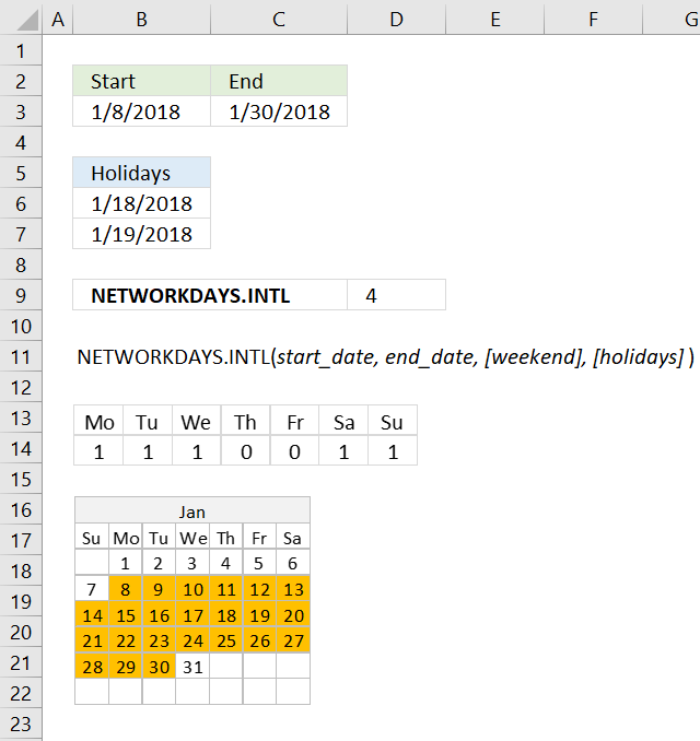
This example demonstrates how to use the NETWORKDAYS.INTL function. The image above shows a date range in cells B3:C3, the start date is 1/8/2018 and the end date is 1/30/2018. The holidays are specified in cells B6 and B7, they are: 1/18/2018 and 1/19/2018. Cells B14:D14 contain a text string where 1 represents "weekend" and 0 (zero) represents "weekday", the text string in this example is "1110011" where the first position represents Monday, the second position represents Tuesday, and so on. The last digit is Sunday. Example, "1110011" considers only Thursdays and Fridays as workdays, all other days in the week are weekend days.
The NETWORKDAYS.INTL function has the following arguments:
- start_date - B3
- end_date - C3
- [weekend] - "1110011"
- [holidays] - B6:B7
Formula in cell D9:
If the start date is 1/8/2018 and the end date is 1/30/2018, 1/18/2018 and 1/19/2018 are holidays then only 1/11/2018, 1/12/2018, 1/25/2018, and 1/26/2018 matches the criteria meaning there are four workdays which is the number displayed in cell D9.
4. NETWORKDAYS.INTL example - count a specific weekday between two dates
NETWORKDAYS function returns the number of whole workdays between two dates, however the formula I am going to demonstrate in this article counts, for example, Mondays or any weekday in a date range. Later in this article, I will show you how to exclude holidays.
Update! I recommend using the NETWORKDAYS.INTL function to count weekdays, it is a lot smaller and easier to work with.
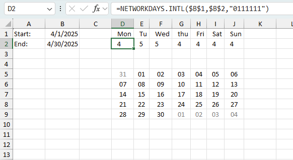
Regular formula in cell D2:
Copy cell D2 and paste to cell range E2:J2. You need to change "0111111" to "1011111" in cell E2, in cell F2 change it to "1101111" and so on.
The text string "0111111" allows you to specify which days are weekdays and which are weekends. There are seven characters and they can be 1 or 0 (zero), 1 indicates it is a weekend and not being counted, 0 (zero) is a weekday.
However, in this case, I am using the string to exclude specific days, I am not using it to define which days are weekends.
4.1 Exclude holidays
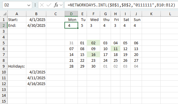
Update! You can use the NETWORKDAYS.INTL function to count weekdays and ignore holidays as well.
Formula in cell D2:
Array formula in cell D7 (old formula):
How to create an array formula
- Select cell D7.
- Paste array formula.
- Press and hold Ctrl + Shift.
- Press Enter.
How to copy array formula
- Copy cell D7.
- Select cell range E7:J7.
- Paste.
5. Count a specific weekday between two dates - alternative formula

This alternative formula is larger and more complicated, I recommend using the NETWORKDAYS.INTL function instead.
Array formula in cell D2 (old formula):
How to create an array formula
- Select cell D2.
- Paste array formula.
- Press and hold Ctrl + Shift simultaneously.
- Press Enter.
- Release all keys.
How to copy array formula
- Copy cell D2.
- Select cell range E2:J2.
- Paste.
Explaining formula in cell D2
Step 1 - Create dates in the date range
$B$1+(ROW($A$1:INDEX($A$1:$A$1000, $B$2-($B$1-1)))-1)
becomes
41000+(ROW($A$1:INDEX($A$1:$A$1000, 41029-(41000-1)))-1)
becomes
41000+(ROW($A$1:INDEX($A$1:$A$1000, 41029-40999))-1)
becomes
41000+(ROW($A$1:INDEX($A$1:$A$1000, 41029-40999))-1)
becomes
41000+(ROW($A$1:INDEX($A$1:$A$1000, 30))-1)
becomes
41000+(ROW($A$1:$A$30)-1)
becomes
41000+({1, 2, 3, 4, 5, 6, 7, 8, 9, 10, 11, 12, 13, 14, 15, 16, 17, 18, 19, 20, 21, 22, 23, 24, 25, 26, 27, 28, 29, 30}-1)
becomes
41000+{0, 1, 2, 3, 4, 5, 6, 7, 8, 9, 10, 11, 12, 13, 14, 15, 16, 17, 18, 19, 20, 21, 22, 23, 24, 25, 26, 27, 28, 29}
and returns
{41000, 41001, 41002, 41003, 41004, 41005, 41006, 41007, 41008, 41009, 41010, 41011, 41012, 41013, 41014, 41015, 41016, 41017, 41018, 41019, 41020, 41021, 41022, 41023, 41024, 41025, 41026, 41027, 41028, 41029}
Step 2 - Convert dates to days of the week
TEXT($B$1+(ROW($A$1:INDEX($A$1:$A$1000, $B$2-($B$1-1)))-1), "ddd")
becomes
TEXT({41000, 41001, 41002, 41003, 41004, 41005, 41006, 41007, 41008, 41009, 41010, 41011, 41012, 41013, 41014, 41015, 41016, 41017, 41018, 41019, 41020, 41021, 41022, 41023, 41024, 41025, 41026, 41027, 41028, 41029}, "ddd")
and returns
{"Sun", "Mon", "Tue", "Wed", "Thu", "Fri", "Sat", "Sun", "Mon", "Tue", "Wed", "Thu", "Fri", "Sat", "Sun", "Mon", "Tue", "Wed", "Thu", "Fri", "Sat", "Sun", "Mon", "Tue", "Wed", "Thu", "Fri", "Sat", "Sun", "Mon"}
Step 3 - Check if values in array are equal to the value in cell D1 (Mon)
IF(TEXT($B$1+(ROW($A$1:INDEX($A$1:$A$1000, $B$2-($B$1-1)))-1), "ddd")=D1, 1, 0)
becomes
IF({"Sun", "Mon", "Tue", "Wed", "Thu", "Fri", "Sat", "Sun", "Mon", "Tue", "Wed", "Thu", "Fri", "Sat", "Sun", "Mon", "Tue", "Wed", "Thu", "Fri", "Sat", "Sun", "Mon", "Tue", "Wed", "Thu", "Fri", "Sat", "Sun", "Mon"}, "ddd")="Mon", 1, 0)
and returns
{0, 1, 0, 0, 0, 0, 0, 0, 1, 0, 0, 0, 0, 0, 0, 1, 0, 0, 0, 0, 0, 0, 1, 0, 0, 0, 0, 0, 0, 1}
Step 4 - Sum values in array
SUMPRODUCT(IF(TEXT($B$1+(ROW($A$1:INDEX($A$1:$A$1000, $B$2-($B$1-1)))-1), "ddd")=D1, 1, 0))
becomes
SUMPRODUCT({0, 1, 0, 0, 0, 0, 0, 0, 1, 0, 0, 0, 0, 0, 0, 1, 0, 0, 0, 0, 0, 0, 1, 0, 0, 0, 0, 0, 0, 1})
and returns 5 in cell D2.
6. Function not working
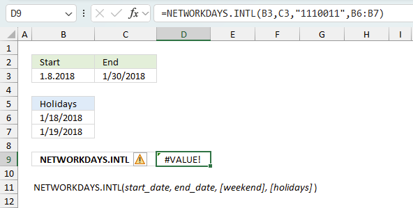
The NETWORKDAYS.INTL function returns a
- #VALUE! error if the arguments contain invalid Excel dates.
- #NAME? error if you misspell the function name.
- propagates errors, meaning that if the input contains an error (e.g., #VALUE!, #REF!), the function will return the same error.
6.1 Troubleshooting the error value
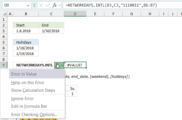
When you encounter an error value in a cell a warning symbol appears, displayed in the image above. Press with mouse on it to see a pop-up menu that lets you get more information about the error.
- The first line describes the error if you press with left mouse button on it.
- The second line opens a pane that explains the error in greater detail.
- The third line takes you to the "Evaluate Formula" tool, a dialog box appears allowing you to examine the formula in greater detail.
- This line lets you ignore the error value meaning the warning icon disappears, however, the error is still in the cell.
- The fifth line lets you edit the formula in the Formula bar.
- The sixth line opens the Excel settings so you can adjust the Error Checking Options.
Here are a few of the most common Excel errors you may encounter.
#NULL error - This error occurs most often if you by mistake use a space character in a formula where it shouldn't be. Excel interprets a space character as an intersection operator. If the ranges don't intersect an #NULL error is returned. The #NULL! error occurs when a formula attempts to calculate the intersection of two ranges that do not actually intersect. This can happen when the wrong range operator is used in the formula, or when the intersection operator (represented by a space character) is used between two ranges that do not overlap. To fix this error double check that the ranges referenced in the formula that use the intersection operator actually have cells in common.
#SPILL error - The #SPILL! error occurs only in version Excel 365 and is caused by a dynamic array being to large, meaning there are cells below and/or to the right that are not empty. This prevents the dynamic array formula expanding into new empty cells.
#DIV/0 error - This error happens if you try to divide a number by 0 (zero) or a value that equates to zero which is not possible mathematically.
#VALUE error - The #VALUE error occurs when a formula has a value that is of the wrong data type. Such as text where a number is expected or when dates are evaluated as text.
#REF error - The #REF error happens when a cell reference is invalid. This can happen if a cell is deleted that is referenced by a formula.
#NAME error - The #NAME error happens if you misspelled a function or a named range.
#NUM error - The #NUM error shows up when you try to use invalid numeric values in formulas, like square root of a negative number.
#N/A error - The #N/A error happens when a value is not available for a formula or found in a given cell range, for example in the VLOOKUP or MATCH functions.
#GETTING_DATA error - The #GETTING_DATA error shows while external sources are loading, this can indicate a delay in fetching the data or that the external source is unavailable right now.
6.2 The formula returns an unexpected value
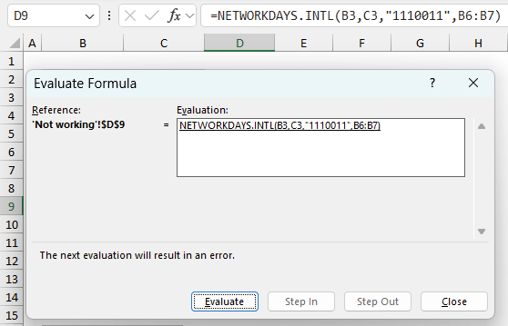
To understand why a formula returns an unexpected value we need to examine the calculations steps in detail. Luckily, Excel has a tool that is really handy in these situations. Here is how to troubleshoot a formula:
- Select the cell containing the formula you want to examine in detail.
- Go to tab “Formulas” on the ribbon.
- Press with left mouse button on "Evaluate Formula" button. A dialog box appears.
The formula appears in a white field inside the dialog box. Underlined expressions are calculations being processed in the next step. The italicized expression is the most recent result. The buttons at the bottom of the dialog box allows you to evaluate the formula in smaller calculations which you control. - Press with left mouse button on the "Evaluate" button located at the bottom of the dialog box to process the underlined expression.
- Repeat pressing the "Evaluate" button until you have seen all calculations step by step. This allows you to examine the formula in greater detail and hopefully find the culprit.
- Press "Close" button to dismiss the dialog box.
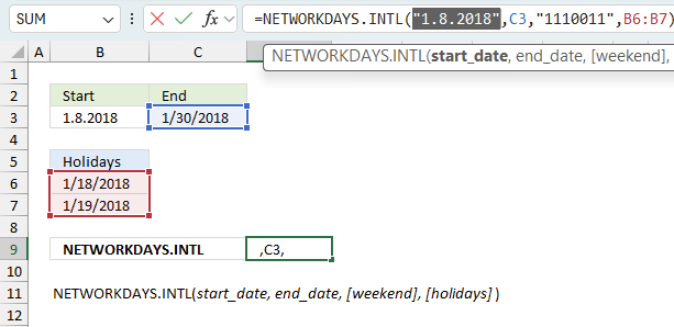
There is also another way to debug formulas using the function key F9. F9 is especially useful if you have a feeling that a specific part of the formula is the issue, this makes it faster than the "Evaluate Formula" tool since you don't need to go through all calculations to find the issue..
- Enter Edit mode: Double-press with left mouse button on the cell or press F2 to enter Edit mode for the formula.
- Select part of the formula: Highlight the specific part of the formula you want to evaluate. You can select and evaluate any part of the formula that could work as a standalone formula.
- Press F9: This will calculate and display the result of just that selected portion.
- Evaluate step-by-step: You can select and evaluate different parts of the formula to see intermediate results.
- Check for errors: This allows you to pinpoint which part of a complex formula may be causing an error.
The image above shows cell reference B3 converted to hard-coded value using the F9 key. The NETWORKDAYS.INTL function requires a valid Excel date which is not the case in this example. We have found what is wrong with the formula.
Tips!
- View actual values: Selecting a cell reference and pressing F9 will show the actual values in those cells.
- Exit safely: Press Esc to exit Edit mode without changing the formula. Don't press Enter, as that would replace the formula part with the calculated value.
- Full recalculation: Pressing F9 outside of Edit mode will recalculate all formulas in the workbook.
Remember to be careful not to accidentally overwrite parts of your formula when using F9. Always exit with Esc rather than Enter to preserve the original formula. However, if you make a mistake overwriting the formula it is not the end of the world. You can “undo” the action by pressing keyboard shortcut keys CTRL + z or pressing the “Undo” button
6.3 Other errors
Floating-point arithmetic may give inaccurate results in Excel - Article
Floating-point errors are usually very small, often beyond the 15th decimal place, and in most cases don't affect calculations significantly.
'NETWORKDAYS.INTL' function examples
Functions in 'Date and Time' category
The NETWORKDAYS.INTL function function is one of 22 functions in the 'Date and Time' category.
Excel function categories
Excel categories
3 Responses to “How to use the NETWORKDAYS.INTL function”
Leave a Reply
How to comment
How to add a formula to your comment
<code>Insert your formula here.</code>
Convert less than and larger than signs
Use html character entities instead of less than and larger than signs.
< becomes < and > becomes >
How to add VBA code to your comment
[vb 1="vbnet" language=","]
Put your VBA code here.
[/vb]
How to add a picture to your comment:
Upload picture to postimage.org or imgur
Paste image link to your comment.
Oscar, here's an alternative
=SUM(--(TEXT(ROW(INDIRECT("A"&$B$1&":A"&$B$2)),"ddd")=D1)) for the first formula
My alternative for the 2nd Formula (excluding the holidays)
=SUM(IF(NOT(ISNUMBER(MATCH(ROW(INDIRECT("A"&$B$1&":A"&$B$2)),Holidays,0))),(--(TEXT(ROW(INDIRECT("A"&$B$1&":A"&$B$2)),"ddd")=D1))))
chrisham,
Yes, thanks.
I seem to have answered this question already, here is also an alternative:
How many of a specific weekday falls between a start date and an end date except holidays