How to use the DAY function
What is the DAY function?
The DAY function extracts the day as a number from an Excel date.
Table of Contents
1. Syntax
DAY(serial_number)
2. Arguments
| serial_number | Required. The Excel date value you want to extract the day number from. |
Excel dates are actually numbers formatted as dates. January 1, 1900 is serial number 1, and January 1, 2008 is serial number 39448 because it is 39,448 days after January 1, 1900.
3. Example
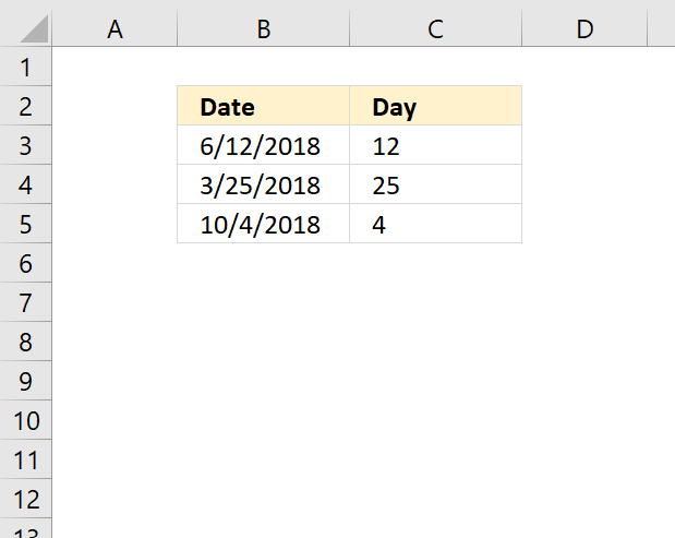
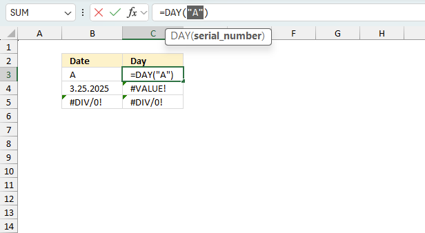
The image above demonstrates a formula in cell C3 that extracts the day number from a date, however, the date must be an Excel date.
Formula in cell C3:
To understand the DAY function I need to explain that it needs an Excel date in order to calculate the day properly. The date in cell B3 is an Excel date meaning it is a number formatted as a date. 1 is 1/1/1900 and 1/1/2000 is 36526 meaning there are 36526 days between the dates.
You can verify this, select a cell containing 1/1/2000 and press CTRL + 1 to open the "Format Cells" dialog box.

4. Function not working
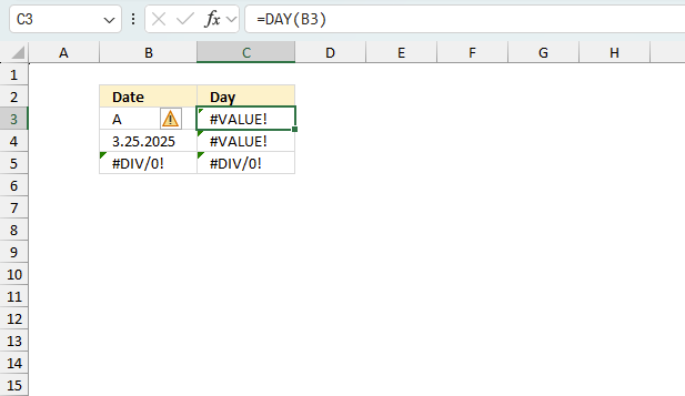
The DAY function returns
- #VALUE! error if you use a non-numeric input value.
- #NAME? error if you misspell the function name.
- propagates errors, meaning that if the input contains an error (e.g., #VALUE!, #REF!), the function will return the same error.
How do I know the date is recognized as an Excel date?
Check the "Format Cells" dialog box and press with left mouse button on category "General". You should see a number and not a date.
How do I convert a date to an Excel date?
Try using the DATEVALUE function to convert a text date to an Excel date. Read this article if it is not working.
4.1 Troubleshooting the error value
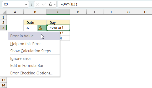
When you encounter an error value in a cell a warning symbol appears, displayed in the image above. Press with mouse on it to see a pop-up menu that lets you get more information about the error.
- The first line describes the error if you press with left mouse button on it.
- The second line opens a pane that explains the error in greater detail.
- The third line takes you to the "Evaluate Formula" tool, a dialog box appears allowing you to examine the formula in greater detail.
- This line lets you ignore the error value meaning the warning icon disappears, however, the error is still in the cell.
- The fifth line lets you edit the formula in the Formula bar.
- The sixth line opens the Excel settings so you can adjust the Error Checking Options.
Here are a few of the most common Excel errors you may encounter.
#NULL error - This error occurs most often if you by mistake use a space character in a formula where it shouldn't be. Excel interprets a space character as an intersection operator. If the ranges don't intersect an #NULL error is returned. The #NULL! error occurs when a formula attempts to calculate the intersection of two ranges that do not actually intersect. This can happen when the wrong range operator is used in the formula, or when the intersection operator (represented by a space character) is used between two ranges that do not overlap. To fix this error double check that the ranges referenced in the formula that use the intersection operator actually have cells in common.
#SPILL error - The #SPILL! error occurs only in version Excel 365 and is caused by a dynamic array being to large, meaning there are cells below and/or to the right that are not empty. This prevents the dynamic array formula expanding into new empty cells.
#DIV/0 error - This error happens if you try to divide a number by 0 (zero) or a value that equates to zero which is not possible mathematically.
#VALUE error - The #VALUE error occurs when a formula has a value that is of the wrong data type. Such as text where a number is expected or when dates are evaluated as text.
#REF error - The #REF error happens when a cell reference is invalid. This can happen if a cell is deleted that is referenced by a formula.
#NAME error - The #NAME error happens if you misspelled a function or a named range.
#NUM error - The #NUM error shows up when you try to use invalid numeric values in formulas, like square root of a negative number.
#N/A error - The #N/A error happens when a value is not available for a formula or found in a given cell range, for example in the VLOOKUP or MATCH functions.
#GETTING_DATA error - The #GETTING_DATA error shows while external sources are loading, this can indicate a delay in fetching the data or that the external source is unavailable right now.
4.2 The formula returns an unexpected value
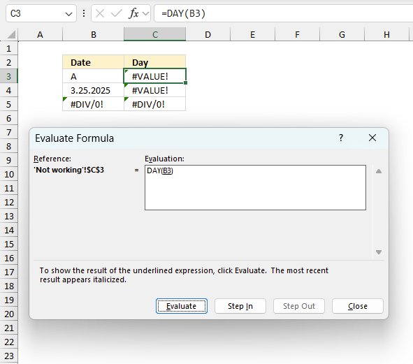
To understand why a formula returns an unexpected value we need to examine the calculations steps in detail. Luckily, Excel has a tool that is really handy in these situations. Here is how to troubleshoot a formula:
- Select the cell containing the formula you want to examine in detail.
- Go to tab “Formulas” on the ribbon.
- Press with left mouse button on "Evaluate Formula" button. A dialog box appears.
The formula appears in a white field inside the dialog box. Underlined expressions are calculations being processed in the next step. The italicized expression is the most recent result. The buttons at the bottom of the dialog box allows you to evaluate the formula in smaller calculations which you control. - Press with left mouse button on the "Evaluate" button located at the bottom of the dialog box to process the underlined expression.
- Repeat pressing the "Evaluate" button until you have seen all calculations step by step. This allows you to examine the formula in greater detail and hopefully find the culprit.
- Press "Close" button to dismiss the dialog box.
There is also another way to debug formulas using the function key F9. F9 is especially useful if you have a feeling that a specific part of the formula is the issue, this makes it faster than the "Evaluate Formula" tool since you don't need to go through all calculations to find the issue..
- Enter Edit mode: Double-press with left mouse button on the cell or press F2 to enter Edit mode for the formula.
- Select part of the formula: Highlight the specific part of the formula you want to evaluate. You can select and evaluate any part of the formula that could work as a standalone formula.
- Press F9: This will calculate and display the result of just that selected portion.
- Evaluate step-by-step: You can select and evaluate different parts of the formula to see intermediate results.
- Check for errors: This allows you to pinpoint which part of a complex formula may be causing an error.
The image above shows cell reference B3 converted to hard-coded value using the F9 key. The DAY function requires numerical values which is not the case in this example. We have found what is wrong with the formula.
Tips!
- View actual values: Selecting a cell reference and pressing F9 will show the actual values in those cells.
- Exit safely: Press Esc to exit Edit mode without changing the formula. Don't press Enter, as that would replace the formula part with the calculated value.
- Full recalculation: Pressing F9 outside of Edit mode will recalculate all formulas in the workbook.
Remember to be careful not to accidentally overwrite parts of your formula when using F9. Always exit with Esc rather than Enter to preserve the original formula. However, if you make a mistake overwriting the formula it is not the end of the world. You can “undo” the action by pressing keyboard shortcut keys CTRL + z or pressing the “Undo” button
4.3 Other errors
Floating-point arithmetic may give inaccurate results in Excel - Article
Floating-point errors are usually very small, often beyond the 15th decimal place, and in most cases don't affect calculations significantly.
5.1 DAY function alternative - TEXT function

Formula in cell C3:
5.1.1 Explaining formula
Step 1 - TEXT function
The TEXT function lets you format values.
TEXT(value, format_text)
value - The string you want to format. You can use a cell reference here or use a text string.
format_text - Formatting code allowing you to change the way, for example, a date or a number is displayed to the Excel user.
Step 2 - Populate arguments
The TEXT function has two arguments.
value - B3
format_text - "d"
"d" is an abbreviation for day. A single "d" returns the day like this: 1. A double "dd" returns 01.
Check out this article to learn more about formatting codes in the TEXT function.
Step 3 - Evaluate TEXT function
TEXT(B3, "d")
becomes
TEXT(43263, "d")
and returns 12.
5.2 DAY function alternative - Cell formatting

You can also show the day number using cell formatting, the image above shows cell formatting applied to cell C5.
How to apply cell formatting:
- Select cell C3.
- Press CTRL + 1 to open the "Format Cells" dialog box.
- Press with left mouse button on "Category" Custom, see the image above.
- Enter d below Type:
- Press with left mouse button on the OK button to apply changes.
6. Filter dates based on a given day number

Formula in cell D3:
Explaining formula
Step 1 - Calculate day number for each date value
DAY(B3:B11)
becomes
DAY({44667; 44667; 44700; 44707; 45006; 45051; 45054; 45075; 45079})
and returns
{16; 15; 16; 26; 16; 16; 8; 29; 16}.
Step 2 - Compare month number to condition
The equal sign lets you check if values are equal, note that this does not perform a case-sensitive comparison. Check out the EXACT function if upper and lower letters matter.
DAY(B3:B11)=16
becomes
{16; 15; 16; 26; 16; 16; 8; 29; 16}=16
and returns
{TRUE; FALSE; TRUE; FALSE; TRUE; TRUE; FALSE; FALSE; TRUE}.
Step 3 - Extract dates meeting the condition
The FILTER function is a new function available to Excel 365 subscribers. It lets you extract values based on a condition or criteria.
FILTER(array, include, [if_empty])
FILTER(B3:B11, DAY(B3:B11)=16)
becomes
FILTER({44667; 44667; 44700; 44707; 45006; 45051; 45054; 45075; 45079}, {TRUE; FALSE; TRUE; FALSE; TRUE; TRUE; FALSE; FALSE; TRUE})
and returns
{44667; 44700; 45006; 45051; 45079}.
7. Create a dynamic calendar using the DAY function

The formula in cell B4 is a dynamic array formula and works only in Excel 365. The SEQUENCE function is only available to Excel 365 subscribers.
The formula uses the provided date in cell B2 to calculate all dates for that month. Make sure you only use Excel dates in cell B2 and that the date is the first date in any given month.
The dates in B4:H9 automatically refresh as soon as a new date is entered in cell B2, this is why it is called a dynamic calendar.
Excel 365 formula in cell B4:
Explaining formula
The dynamic array formula in cell B4 is entered as a regular formula, however, it spills values to the right and below as far as needed.
Make sure the adjacent cells are empty or a #SPILL! error is shown.
Step 1 - Calculate weekday
This step is needed in order to calculate the first date in the week, it is most often not the same date as the first date in a month. It is the 27th in this example, shown in the image above.
The WEEKDAY function returns a number representing the weekday in a week. 1 - Sunday, 2 - Monday, and so on.
WEEKDAY(serial_number,[return_type])
WEEKDAY(B2,1)
becomes
WEEKDAY(44621, 1)
and returns 3. This means that March the 1st, 2022 is a Tuesday.
Step 2 - Create an array large enough to populate a monthly calendar
The SEQUENCE function creates a list of sequential numbers to a cell range or array. It is located in the Math and trigonometry category and is only available to Excel 365 subscribers.
SEQUENCE(rows, [columns], [start], [step])
SEQUENCE(6,7)
returns
{1, 2, 3, 4, 5, 6, 7; 8, 9, 10, 11, 12, 13, 14; 15, 16, 17, 18, 19, 20, 21; 22, 23, 24, 25, 26, 27, 28; 29, 30, 31, 32, 33, 34, 35; 36, 37, 38, 39, 40, 41, 42}.
Note the delimiting characters used in the array above, the comma separates values between columns and the semicolon between rows. Your setup may use other delimiting characters, you can change these in the regional settings.
Step 3 - Calculate the date for the first sunday
This is often a date in the previous month. The plus and minus sign lets you perform arithmetic calculations in an Excel formula.
B2-WEEKDAY(B2,1)+SEQUENCE(6,7)
becomes
44621 - 3 + {1, 2, 3, 4, 5, 6, 7; 8, 9, 10, 11, 12, 13, 14; 15, 16, 17, 18, 19, 20, 21; 22, 23, 24, 25, 26, 27, 28; 29, 30, 31, 32, 33, 34, 35; 36, 37, 38, 39, 40, 41, 42}
and returns
{44619, 44620, 44621, 44622, 44623, 44624, 44625; 44626, 44627, 44628, 44629, 44630, 44631, 44632; 44633, 44634, 44635, 44636, 44637, 44638, 44639; 44640, 44641, 44642, 44643, 44644, 44645, 44646; 44647, 44648, 44649, 44650, 44651, 44652, 44653; 44654, 44655, 44656, 44657, 44658, 44659, 44660}
Step 4 - Calculate the day for each date in the array
DAY(B2-WEEKDAY(B2,1)+SEQUENCE(6,7))
becomes
DAY({44619, 44620, 44621, 44622, 44623, 44624, 44625; 44626, 44627, 44628, 44629, 44630, 44631, 44632; 44633, 44634, 44635, 44636, 44637, 44638, 44639; 44640, 44641, 44642, 44643, 44644, 44645, 44646; 44647, 44648, 44649, 44650, 44651, 44652, 44653; 44654, 44655, 44656, 44657, 44658, 44659, 44660})
and returns
{27, 28, 1, 2, 3, 4, 5; 6, 7, 8, 9, 10, 11, 12; 13, 14, 15, 16, 17, 18, 19; 20, 21, 22, 23, 24, 25, 26; 27, 28, 29, 30, 31, 1, 2; 3, 4, 5, 6, 7, 8, 9}.
'DAY' function examples
Table of Contents Automate net asset value (NAV) calculation on your stock portfolio Calculate your stock portfolio performance with Net […]
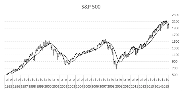
In my previous post, I described how to build a dynamic stock chart that lets you easily adjust the date […]
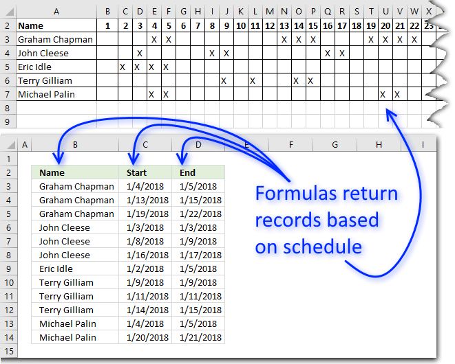
This article demonstrates ways to extract names and corresponding populated date ranges from a schedule using Excel 365 and earlier […]
Functions in 'Date and Time' category
The DAY function function is one of 22 functions in the 'Date and Time' category.
How to comment
How to add a formula to your comment
<code>Insert your formula here.</code>
Convert less than and larger than signs
Use html character entities instead of less than and larger than signs.
< becomes < and > becomes >
How to add VBA code to your comment
[vb 1="vbnet" language=","]
Put your VBA code here.
[/vb]
How to add a picture to your comment:
Upload picture to postimage.org or imgur
Paste image link to your comment.
Contact Oscar
You can contact me through this contact form