Populate drop down list with unique distinct values sorted from A to Z
Question:
How do I create a drop-down list with unique distinct alphabetically sorted values?
Table of contents
1. Introduction
What is a drop down list?
A drop-down list is a built-in tool to control the input value for a given cell. It allows you to press with left mouse button on a button next to the selected cell and a list appears populated with valid values you can use.
There are three types of drop-down lists in Excel:
- Regular. To access and deploy a regular drop-down list, go to the "Data" tab on the ribbon. Press with left mouse button on with left mouse button on the "Data Validation" button, a dialog box appears. Select "List" and then the source data range. Press with left mouse button on OK to apply changes.
- Form Control. You will find the drop-down list on tab "Developer" on the ribbon. Press with left mouse button on the "Insert" button and a popup menu appears. Press with mouse on either "Combo box" or "List box". Press with left mouse button on and drag with mouse on the worksheet to create.
- ActiveX. You will find the ActiveX buttons next to the Form Control buttons. See instructions above.
What are unique distinct values?
Unique distinct list has only one value or instance from a source dataset. In other words, duplicate values are merged into one distinct value.
Example:
- Dataset: [2, 3, 3, 4, 5, 5, 6]
- Unique Distinct values: [2, 3, 4, 5, 6]
What is VBA?
VBA (Visual Basic for Applications) is a programming language developed by Microsoft that is used for automating tasks in Microsoft Office applications such as Excel, Word, and Access. It allows users to create macros, automate repetitive tasks, and enhance Office functionality with custom scripts.
How to enable developer tab?
Here is how to enable the "Developer" tab if it is missing on the ribbon:
- Press with left mouse button on "File" located above the ribbon, a new pane appears.
- Press with mouse on the "Options" button to access Excel settings.
- Press with mouse on "Customize Ribbon" and then on the right side press with left mouse button on the checkbox next to the tab "Developer" to enable it.
- Press with left mouse button on "OK" button to apply changes.
The "Developer" tab is now visible on the ribbon. Here are instructions for Excel 2007, Excel 2010 and Excel 2013
2. Sort values using array formula
The following example shows how to sort and populate a drop-down list in earlier Excel versions. See section 3 for an Excel 365 formula.
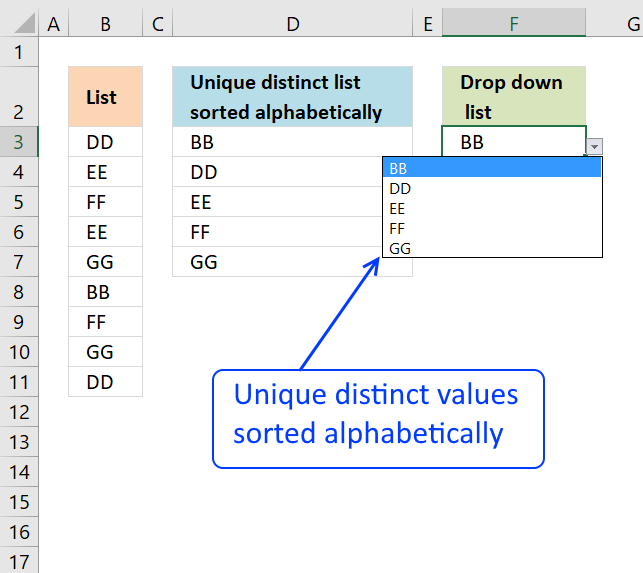
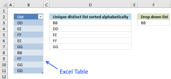
The helper column D filters unique distinct values sorted from A to Z from values in column B. The drop-down list in cell F3 is populated with the values in column D.
Array formula in cell D3
The issues with this formula is:
- The formula needs to be entered as an array formula.
- The formula has to be entered to more cells if the list grows.
- You need to adjust the cell references if the source data list grows or shrinks.
You can convert source data $B$3:$B$11 to an Excel defined Table to remove the need for adjusting cell references when data is added or removed.
Watch a video explaining the formula
Watch a video explaining how to populate Drop-Down list with a dynamic named range
How to create an array formula
- Select cell D3
- Type above array formula
- Press and hold Ctrl + Shift
- Press Enter once
- Release all keys
How to copy array formula
- Select cell D3
- Copy cell (Ctrl + c)
- Select cell range D4:D7
- Paste (Ctrl + v)
2.1 Explaining array formula in cell D3
Step 1 - Filter unique distinct values
COUNTIF($D$2:D2,$B$3:$B$11)=0
The COUNTIF function counts previous values above to make sure that no duplicates are displayed.
If no values in previous cells above are found the COUNTIF function returns a 0 (zero) for that position in the array.
COUNTIF($D$2:D2,$B$3:$B$11) returns {0;0;0;0;0;0;0;0;0}
COUNTIF($D$2:D2,$B$3:$B$11)=0 returns {TRUE;TRUE; TRUE;TRUE; TRUE;TRUE; TRUE;TRUE;TRUE}
The picture below shows the array in cell range C3:C11. The array tells the formula that no values have yet been displayed in cells above cell D3
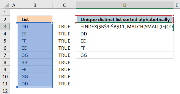
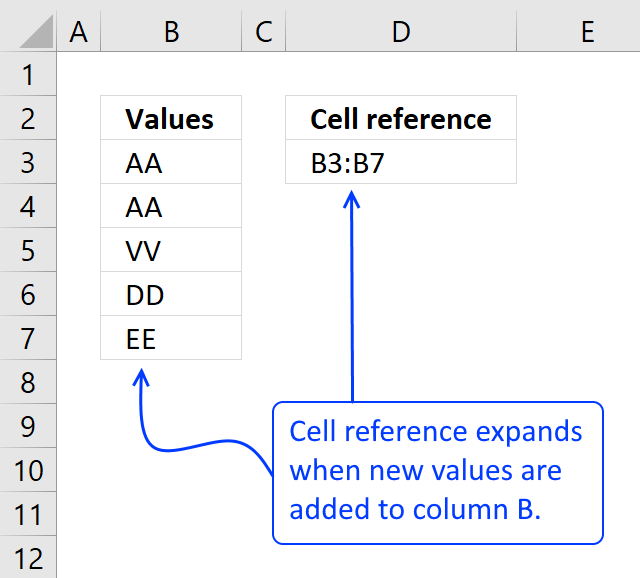
Note that the first argument in the COUNTIF function ($D$2:D2) is a growing cell reference meaning when you copy the formula to cells below the cell reference expands automatically.
Step 2 - Create an array with sort rank numbers
The COUNTIF function comes once again to rescue, it allows you to rank each value in cell range B3:B11 based on its position in a sorted array.
COUNTIF($B$3:$B$11, "<"&$B$3:$B$11)
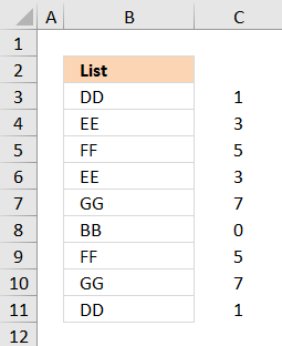
Value "BB" is first in a sorted list indicated by the corresponding value 0 (zero) in column C. The second value is "DD" with rank number 1.
COUNTIF($B$3:$B$11, "<"&$B$3:$B$11) returns {1;3;5;3;7;0;5;7;1}
Step 3 - Build an array with rank numbers based on which values that have not been shown yet
IF(COUNTIF($D$2:D2,$B$3:$B$11)=0,COUNTIF($B$3:$B$11, "<"&$B$3:$B$11),"") returns {1;3;5;3;7;0;5;7;1}
No values in the array have been filtered out, this makes sense since the array formula is in cell D3 and no values have been displayed yet.
Step 4 - Find the smallest value in the array
The SMALL function lets you filter the n-th smallest value from an array of values. It has a major advantage to the MIN function as it also ignores text and blank values.
SMALL(IF(COUNTIF($D$2:D2,$B$3:$B$11)=0,COUNTIF($B$3:$B$11, "<"&$B$3:$B$11),""), 1)
becomes
SMALL({1;3;5;3;7;0;5;7;1}, 1)
and returns 0 (zero).
Step 4 - Find the position of a value in an array of values
To be able to fetch the right value to cell D3 we need to know it's position in column B. The MATCH function returns the position.
MATCH(SMALL(IF(COUNTIF($D$2:D2,$B$3:$B$11)=0,COUNTIF($B$3:$B$11, "<"&$B$3:$B$11),""), 1), COUNTIF($B$3:$B$11, "<"&$B$3:$B$11), 0)
returns 6. Value 0 (zero) is in position 6 in this array {1;3;5;3;7;0;5;7;1}
Step 5 - Fetch value
The INDEX function retrieves a value based on a coordinate, since it is only a column the INDEX function allows you to only use a row number as a coordinate.
INDEX($B$3:$B$11, MATCH(SMALL(IF(COUNTIF($D$2:D2,$B$3:$B$11)=0,COUNTIF($B$3:$B$11, "<"&$B$3:$B$11),""), 1), COUNTIF($B$3:$B$11, "<"&$B$3:$B$11), 0))
returns value "BB" in cell D3.
2.2 How to create a drop-down list that expands with new values automatically
- Press with left mouse button on Data tab
- Press with left mouse button on Data Validation button
- Press with left mouse button on "Data validation..."
- Select List in the "Allow:" window. See picture below.
- Type =OFFSET($B$2, 0, 0, COUNT(IF($B$2:$B$1000="", "", 1)), 1) in the "Source:" window
- Press with left mouse button on OK!

Final note
Convert the data in column B into an excel defined table to make it dynamic. Then you don't need to adjust the cell references in the array formula in column D every time you add or delete values in column B.
Get *.xlsx file
Create a drop down list containing only unique.xlsx
3. Sort values - Excel 365 dynamic array formula
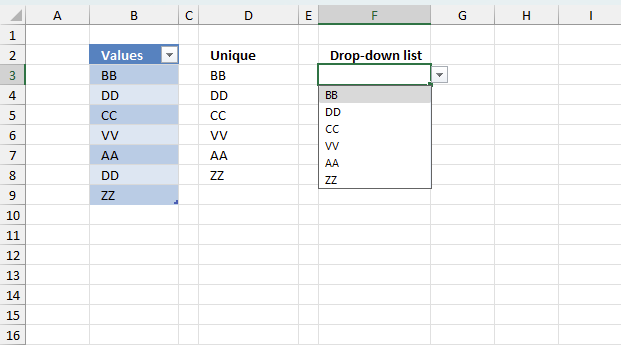
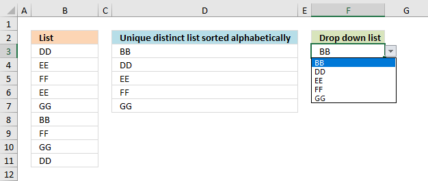
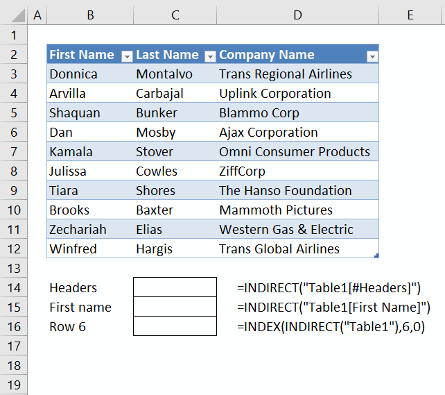
This example shows how to build a drop-down list containing unique distinct values in Excel 365. The image above displays:
- Source range: Cell range B2:B9 is an Excel defined Table. Cells B3:B9 contains values, value "DD" has a duplicate.
- Unique distinct values: Cell D3 contains an Excel 365 dynamic array formula that creates unique distinct values based on cells B3:B9.
- Drop-down list: Cell F3 contains a regular drop-down list populated with values from cell D3 and spilled values below as far as needed.
Excel defined Table
Cell range B2:B9 is an Excel defined Table. It allows you to use a structured reference which is a cell reference that doesn't change when values are added or deleted. The main benefit is that this removes the need for adjusting cell references.
An Excel defined Table is created by selecting a cell in the data you want to convert. Press and hold shortcut key CTRL then press T once. Release all keys.
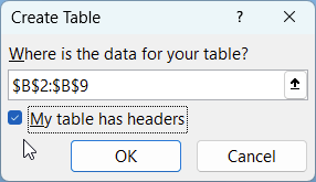
This brings up a dialog box, enable the check box if the data has column header names. Press the OK button to apply the changes.
Excel 365 dynamic array formula
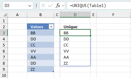
Cell D3 contains the following formula:
The UNIQUE function extracts unique distinct values, the formula spills values to cells below D3 as far as needed. A #SPILL! error is shown if the destination cells are populated.
Table1 is a structured reference meaning a cell reference to the values in Excel Table named Table1. Table1 does not change if values are added, changed or deleted. Table1 points to cell range B3:B9.
Drop-down list
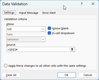
Cell F3 contains a regular drop-down list. It has the following cell reference =D3# in the source field. It is unfortunately not possible to populate the source field with a formula or a named range.
Here is how to access and deploy a regular drop-down lis:
- Go to the "Data" tab on the ribbon.
- Press with left mouse button on with left mouse button on the "Data Validation" button, a dialog box appears. (displayed above)
- Select "List" and then the source data range.
- Press with left mouse button on OK to apply changes.
What Does =D3# Mean?
The # (hashtag) symbol tells Excel to reference the entire spill range starting from D3. A spill range is a dynamic array output from a formula that automatically fills multiple cells in Excel 365. If D3 contains a formula that returns multiple values, it will expand to reference all the spilled values. The # (hashtag) works fine in the source: field in the drop-down list settings dialog box.
4. Sort values using VBA

This exanple shows how to sort and extract unique distinct values from a source range using two user defined functions (udf).
- FilterUniqueSort(rng As Range): This udf uses the SelectingSort function to sort the values from A to Z. Then extracts unique distinct values from the ouput.
- SelectionSort(TempArray As Variant)
The drop-down list in cell D2 is populated with values from cell range B2:B8000.
Array formula in cell B2:B8000:
The advantage of using VBA is that it is often quicker than Excel functions and allows for further customizations.
The downside is that setting it up can be more challenging for inexperienced users, and macro-enabled .xlsm files pose potential security risks, leading many companies to restrict or ban their use.
How to create array formula
Excel 365 users can skip these steps. Simply press Enter after typing the function will make the formula automatically spill values to cells below as far as needed.
- Select cell range B2:B8000.
- Type array formula above.
- Press and hold Ctrl + Shift.
- Press Enter once.
- Release all keys.
VBA code
You can find the selectionsort function here: Using a Visual Basic Macro to Sort Arrays in Microsoft Excel
Function FilterUniqueSort(rng As Range)

Dim ucoll As New Collection, Value As Variant, temp() As Variant
ReDim temp(0)

On Error Resume Next
For Each Value In rng
    If Len(Value) > 0 Then ucoll.Add Value, CStr(Value)
Next Value
On Error GoTo 0

For Each Value In ucoll
    temp(UBound(temp)) = Value
    ReDim Preserve temp(UBound(temp) + 1)
Next Value

ReDim Preserve temp(UBound(temp) - 1)
SelectionSort temp

FilterUniqueSort = Application.Transpose(temp)

End Function


Function SelectionSort(TempArray As Variant)
          Dim MaxVal As Variant
          Dim MaxIndex As Integer
          Dim i, j As Integer

          For i = UBound(TempArray) To 0 Step -1


              MaxVal = TempArray(i)
              MaxIndex = i


              For j = 0 To i
                  If TempArray(j) > MaxVal Then
                      MaxVal = TempArray(j)
                      MaxIndex = j
                  End If
              Next j

              If MaxIndex < i Then
                  TempArray(MaxIndex) = TempArray(i)
                  TempArray(i) = MaxVal
              End If
          Next i

      End Function
Where to copy vba code?
- Press Alt + F11
- Insert a module into your workbook
- Copy (Ctrl + c) above code into the code window
Get excel 97-2003 *,xls file
Create-a-drop-down-list-containing-only-unique_vba.xls
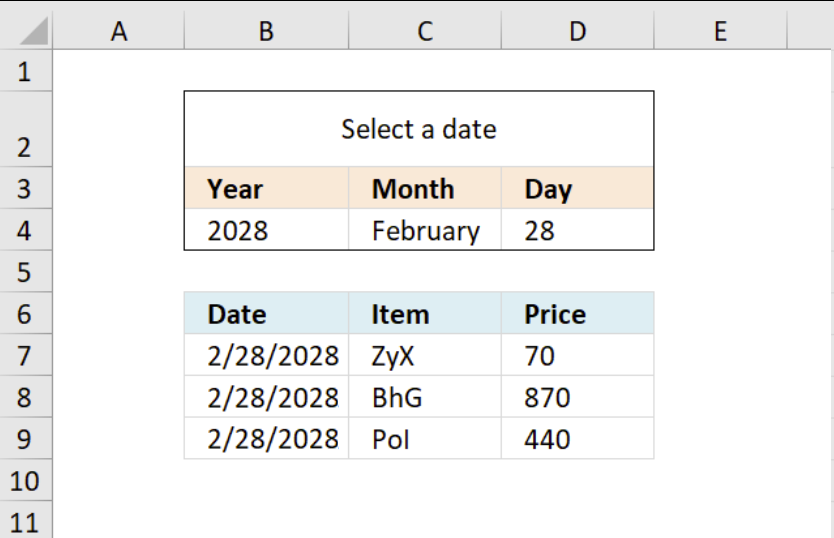
5. Create a drop down calendar
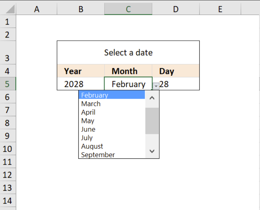
The drop down calendar in the image above uses a "calculation" sheet and a named range. You can copy the drop-down lists and paste anywhere in the workbook but they have to be in the same order and adjacent.
You can select a year and month and a formula calculates the right number of days in the last drop down list, however if you choose "January" and day 31 and then selects February which is possible. The problem is that there are not 31 days in February.
You can use conditional formatting to hide the day when that scenario happens, that will clearly inform the user that the date is not valid. I will show you later in this post how to set it up. Here is how I created the drop down lists:
Create a drop down list for years
- Select cell A1
- Select tab "Data" on the ribbon
- Press with left mouse button on "Data Validation" button
- Press with left mouse button on "Data Validation..."
- Select tab "Settings"
- Select List in "Allow:" drop down list
- Type in "Source:" window
2011, 2012, 2013, 2014, 2015
- Press with left mouse button on OK!
Create a drop down list for months
- Select cell B1
- Select tab "Data" on the ribbon
- Press with left mouse button on "Data Validation" button
- Press with left mouse button on "Data Validation..."
- Select tab "Settings"
- Select List in "Allow:" drop down list
- Type in "Source:" window
January, February, March, April, May, June, July, August, September, October, November, December
- Press with left mouse button on OK!
Recommended articles
Question: How do I create a drop-down list with unique distinct alphabetically sorted values? Table of contents Introduction Sort values […]
Setup Sheet2
- Select sheet2
- Select cell A1
- Type
=row()
in cell A1 and then press ENTER
- Copy cell A1 and paste down to cell A31
Create a named range
- Select tab "Formulas" on the ribbon
- Press with left mouse button on "Name Manager" button
- Press with left mouse button on "New..." button
- Type
days
in Name: window
- Type formula:
=Sheet2!$A$1:INDEX(Sheet2!$A$1:$A$31, DAY(DATE(Sheet1!A1, MATCH(Sheet1!B1, {"January", "February", "March", "April", "May", "June", "July", "August", "September", "October", "November", "December"}, 0)+1, 1)-1))
in "Refers to:" window
- Press with left mouse button on Close button
Recommended articles
What is a named range? A named range is a feature in Excel that allows you to assign a specific […]
Create a drop down list for days
- Select cell C1
- Select tab "Data" on the ribbon
- Press with left mouse button on "Data Validation" button
- Press with left mouse button on "Data Validation..."
- Select tab "Settings"
- Select List in "Allow:" drop down list
- Type in "Source:" window:
=days
- Press with left mouse button on OK!
How to create a list of drop down calendars
- Copy cell A1:C1
- Paste down as far as needed.
The named range is dynamic, all drop down lists in each row is connected.
Hide day if date is invalid
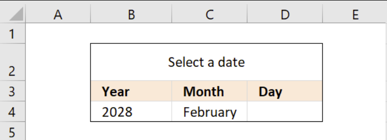
The image above shows what happens if an invalid date is selected, conditional formatting hides the day to alert the user that the date is invalid. The formula in cell J2 checks if the date is valid or not.
- FALSE = Invalid
- TRUE = Valid.
Formula in cell J2:
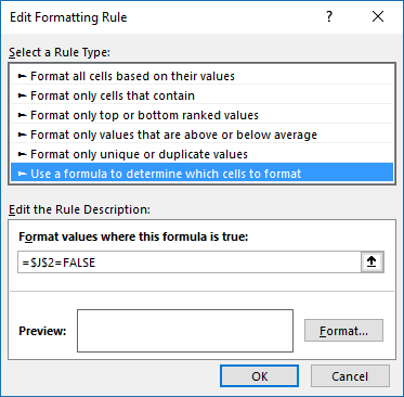
The conditional formatting formula:
How to apply conditional formatting to cell D4
- Select cell D4
- Go to tab "Home" on the ribbon
- Press with left mouse button on "Conditional formatting" button
- Press with left mouse button on "New Rule..."
- Press with mouse on "Use a formula to determine which cells to format"
- Type the formula above in "Format values where this formula is true:"
- Press with left mouse button on "Format" button.
- Press with left mouse button on tab "Font"
- Pick font color white.
- Press with left mouse button on OK
- Press with left mouse button on OK
Example
The image above demonstrates how to filter a table using the date picker and an array formula.
Array formula in cell B7:
To enter an array formula, type the formula in a cell then press and hold CTRL + SHIFT simultaneously, now press Enter once. Release all keys.
The formula bar now shows the formula with a beginning and ending curly bracket telling you that you entered the formula successfully. Don't enter the curly brackets yourself.
Copy cell B7 and paste to cell range B7:D9.
Drop down lists category
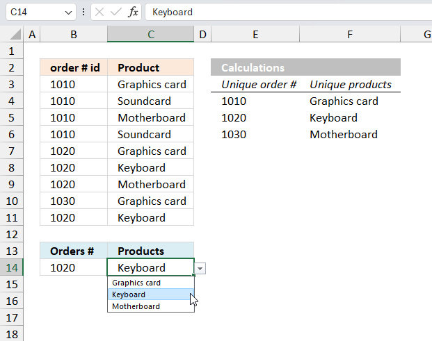
Table of Contents Create dependent drop down lists containing unique distinct values - Excel 365 Create dependent drop down lists […]
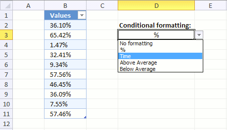
Table of contents How to change cell formatting using a Drop Down list Highlight cells based on coordinates Highlight every […]
This article demonstrates different ways to reference an Excel defined Table in a drop-down list and Conditional Formatting formulas. The […]
Excel categories
84 Responses to “Populate drop down list with unique distinct values sorted from A to Z”
Leave a Reply
How to comment
How to add a formula to your comment
<code>Insert your formula here.</code>
Convert less than and larger than signs
Use html character entities instead of less than and larger than signs.
< becomes < and > becomes >
How to add VBA code to your comment
[vb 1="vbnet" language=","]
Put your VBA code here.
[/vb]
How to add a picture to your comment:
Upload picture to postimage.org or imgur
Paste image link to your comment.
I encountered an issue when using Excel 2007 where upon saving the workbook as an Excel Workbook (not 97-2003) the embedded count(if( ...)) formula causes only the first item in the drop down list to appear. This only happens upon opening the workbook and if you select data validation on the cell the issue is resolved. However, upon saving and reopening the problem reappears. The only workaround if to either remove the function or keep the workbook in 97-2003 format.
For a workaround in excel 2007, you can use the following in the "Refers to:" field under the name manager: =OFFSET($B$2, 0, 0, COUNTIFS($B$2:$B$1000,"",$B$2:$B$1000,"#N/A"), 1)
<
Sorry, it got coruppted. Here is the correct one: For a workaround in excel 2007, you can use the following in the "Refers to:" field under the name manager: =OFFSET($B$2, 0, 0, COUNTIFS($B$2:$B$1000,"<>",$B$2:$B$1000,"<>#N/A"), 1)
Sorry again. Use the above furmula for the data validation. NOT for the name manager.
Josh, thanks for bringing this to my attention. I´ll try to solve this issue.
I want the drop down box to be on a different worksheet. But EXCEL won't allow OFFSET without having it all on one worksheet.
Is there some other way to have the lists on one sheet, get unique values and sort them, then reference them from a drop down on another worksheet? To make matter more fun, I need the ranges to be dynamic as the user may be adding new records.
Thanks!
Dianne
I have re-created the above formula but would like to create a range that is larger than the current data so that the unique list picks up all new data. Currently my unique list repeats the last line of data several times because the range name extends beyond it. Can this be done?
Thanks
Keels
Dianne,
I want the drop down box to be on a different worksheet. But EXCEL won't allow OFFSET without having it all on one worksheet.
It is not OFFSET, it is Data Validation that won´t allow having it all on one worksheet.
But there is a workaround, if you create another named range (for example, named unique) and type =OFFSET(Sheet1!$B$2, 0, 0, COUNT(IF(Sheet1!$B$2:$B$1000="", "", 1)), 1).
Create a drop down box on another sheet and type =unique in "source:"
To make matter more fun, I need the ranges to be dynamic as the user may be adding new records.
I have updated the post, the named range is now dynamic.
Keels,
I have re-created the above formula but would like to create a range that is larger than the current data so that the unique list picks up all new data. Currently my unique list repeats the last line of data several times because the range name extends beyond it. Can this be done?
I have updated this post, the named range is now dynamic.
@Oscar,
Here is a shorter Name Range formula that appears to work the same as the one you posted...
=Sheet2!$A$1:INDEX(Sheet2!$A$1:$A$31, DAY(DATE(Sheet1!$A$1, MONTH(Sheet1!$B$1&1)+1, 0)))
As a side note, you can change the $A$30000 reference in your posted Named Range formula to $A$31 and it will work just as well.
Rick Rothstein (MVP - Excel),
Thanks!!
This is almost exactly what I have been looking for. The only shortcoming is that I need it to work with spaces (empty cells) in the source list and able to handle a source list that is only one item. I want the person to begin to fill out a column (the source list) filling in names and as they go they can instead pick from a drop down menu so they do not have to type the name (and so the name is always the same). When they type the first name in, it does not appear in the list. Only when they type the second name, then both names appear. Can this be fixed? They are allowed to skip rows filling out the table, so handling blank cells is important too. Thank you.
Peter,
Array formula to remove blanks in blog post example:
=INDEX(List, MATCH(0, IF(MAX((COUNTIF($B$1:B1, $A$2:$A$15)=0)*(($A$2:$A$15<>"")*(COUNTIF($A$2:$A$15, ">"&$A$2:$A$15)+1)))=(IF(($A$2:$A$15<>""), COUNTIF($A$2:$A$15, ">"&$A$2:$A$15)+1, "")), 0, ""), 0)) + CTRL + SHIFT + ENTER
I dont´t understand this:
I want the person to begin to fill out a column (the source list) filling in names and as they go they can instead pick from a drop down menu so they do not have to type the name (and so the name is always the same). When they type the first name in, it does not appear in the list. Only when they type the second name, then both names appear. Can this be fixed?
That revised formula worked perfectly. It solved both the problem with spaces interspersed in the source list and the diminutive situation with only one item in the source list (yielding a one item menu). I can't see any reason someone would not prefer this revised equation over the original. I would update your example above to use this formula instead.
As for my explanation as to what I am doing..... sorry that was clear as mud....
I want a column of data entry cells on a form that allows either free form text entry or a dynamic drop down menu of the items the person already typed into that same column. This way they don't have to "type" the same name twice (can pick it from the menu the second time). It makes data entry faster and increases the likely hood that multiple duplicate entries will be the exact same. To allow text entry at the same time as menu selection, I just turn off the data validation error message.
Over time I may build a dynamic list of names from past times the form was filled out so that this drop down menu does not start out blank each time. But right now this is still helpful to the user (and me).
Thank you very much.... I have yet to figure out how all these complex array formulas work. Right now you are the magician and I am the kid in awe.
Peter,
Maybe you can use these instructions:
Excel Data Validation -- Hide Previously Used Items in Dropdown and modify formulas to only show previously used items in a drop down list.
Thanks Oscar,
That might come in handy some day. In the process of scoping that out I stumbled on a bunch of other potentially useful data validation methods including selecting multiple items from a menu.
"If God didn't invent Excel, I bet that's where he spends most of his time." - Peter V.
This is really good; thanks for posting.
Chris,
thank you!
may i ask the maximum limit on the amount of records you can have in a dropdown list?
thanks.
Juna,
I can´t enter more than 32767 values in a drop down list in excel 2007.
Maybe someone else can shed some light on this, I can´t find anything about this (google).
tnx oscar for this formula
but i have a problem with that.
it has to calculate about 8000 cells and it slows down my pc badly.
any suggestions?
luka,
I have updated this article with a vba function. Get the the attached file!
Hi
The dropdown unique listing is really helpful and i appreciate that.
Eddy Stanley,
Thanks!
Hi,
I have a requirement (read problem). I have created a drop down list with following items:
1.Above
2.Below
3.At par
I want if someone choose Above, a formula for escalation of value is executed, if Below a formula for Degradation of value, if At par is used no change in the value.
I am unable to link the chosen field in formula.
Kindly help.
Thanks
DJ,
I am not sure that is possible. What is the formula for escalation of a value?
I would suggest a spin button (form control) and link the control to a cell.
I have a problem if in Column A i have only one value 'DD' (means A1 as List and A2 as DD) then no value are coming in column B using
=INDEX(List, MATCH(0, IF(MAX(NOT(COUNTIF($B$1:B1, List))*(COUNTIF(List, ">"&List)+1))=(COUNTIF(List, ">"&List)+1), 0, 1), 0))
Can u plz give me the fix to it. I am also trying but not sure about it.
This is urgent..
Nidhi,
For some reason that I don´t understand, the dynamic named range used in a function returns an error when the List contains a single value.
I am not sure how to resolve this, maybe you can use a - or # character in the first cell and "DD" in the second cell?
Oscar,
Great work and a huge time saver!!! Thank you.
[quote]For some reason that I don´t understand, the dynamic named range used in a function returns an error when the List contains a single value.[/quote]
It has to do with the way Excel evaluates expressions. When you have only one value, Excel reduces the expressions for the "range" inside of Match as a single unique value, rather than a range of values with only one element in it. Since Match expects its second argument to be a range, then it throws the error.
Example:
The way we'd like Excel to evaluate the "Match" expressions would be:
=MATCH(0, {0},0)
Instead, Excel evaluates it as (note the second argument is plainly "0", a number, and not the array {0}:
=MATCH(0, 0,0)
To correct this, one can force Excel to calculate the result of the "if" as an array, as follows (note the "{0}+" part):
=INDEX(List,MATCH(0,{0}+IF(MAX(NOT(COUNTIF($B$1:B1,List))*(COUNTIF(List,">"&List)+1))=(COUNTIF(List,">"&List)+1),0,1),0))
Hope this helps
Mijael,
Thanks for your valuable contribution!
Another, "one-row-code", VBA tip:
Sub MakeUniqueList()
    Range("A1:A10").AdvancedFilter Action:=xlFilterCopy, _
    CopyToRange:=Range("B1"), Unique:=True
End Sub
!!! Only be aware, that the value from the first line will be taken as the title.
Palo
Thank you so much Oscar. This is really great esp. the explanation of the formulae !
Many thanks for the COUNTIF trick, Oscar. This helps me a lot.
I would change it in a shorter formula, and it works.
=INDEX(List, MATCH((COUNTIF(List, ">"&List)+1), MAX(NOT(COUNTIF($B$1:B1, List))*(COUNTIF(List, ">"&List)+1), 0))
If the data contains all numbers, I will use rank(list,list) to replace (COUNTIF(List, ">"&List)+1)
=INDEX(List, MATCH(RANK(List,List), MAX(NOT(COUNTIF($B$1:B1, List))*RANK(List,List), 0))
sorry, I made a mistake.
I would change it in a shorter formula, and it works.
=INDEX(List, MATCH(MAX(NOT(COUNTIF($B$1:B1, List))*(COUNTIF(List, ">"&List)+1)), (COUNTIF(List, ">"&List)+1), 0))
If the data contains all numbers, I will use rank(list,list) to replace (COUNTIF(List, ">"&List)+1)
=INDEX(List, MATCH(MAX(NOT(COUNTIF($B$1:B1, List))*RANK(List,List)), RANK(List,List), 0))
i can't understand this6
=Sheet2!$A$1:29 ---->> not working
29=INDEX(Sheet2!$A$1:$A$30000,DAY(DATE(Sheet1!A1,MATCH(Sheet1!B1,{"January";"February";"March";"April";"May";"June";"July";"August";"September";"October";"November";"December"},0)+1,1)-1))
Try this formula:
The formula creates a cell reference to sheet 2, column A. The drop down list is then populated with values from sheet2, column A.
Please ....
[...] Names -- Excel Named Ranges Excel Magic Trick # 259: Dynamic DV List Based On DV List - YouTube Create a drop down list containing only unique distinct alphabetically sorted text values using exce... I hope these help and good luck with your project. [...]
[...] OFFSET or Table Feature? - YouTube excelisfun -- Excel How To Videos - YouTube Or here.... Create a drop down list containing only unique distinct alphabetically sorted text values using exce... For Question 2, you can concatenate (join) your two cells and use a Conditional Formatting [...]
Dear Oscar,
Can you help me to get the values of Unique distinct list sorted alphabetically in horizantally instead of vertical by using VBA fuction. Kindly find the eclosed Excel sheet obtained from your website.
Thanks
Sudhakar
Sudhakar,
Function FilterUniqueSort(rng As Range) Dim ucoll As New Collection, Value As Variant, temp() As Variant ReDim temp(0) On Error Resume Next For Each Value In rng If Len(Value) > 0 Then ucoll.Add Value, CStr(Value) Next Value On Error GoTo 0 For Each Value In ucoll temp(UBound(temp)) = Value ReDim Preserve temp(UBound(temp) + 1) Next Value ReDim Preserve temp(UBound(temp) - 1) SelectionSort temp FilterUniqueSort = temp End FunctionMr. Oscar
Thanks for your great help,
cheers...
Sudhakar
Hi. talking about duplicates, I have a problem with that.
I have two arrays to compare and highlight duplicates, I already try -countif conditional formatting-, -index match-, =and, and nothing work my arrays are Number one is A1:F53 and Number two H1:M53 as a little illustration here you are.
10-11-12-17-28-46 against 2-10-11-41-42-53
03-09-11-21-24-49 against 3-13-42-47-52-53
thanks.
vicktor schausberger,
Here is an example:
Conditional formatting formula:
=COUNTIF($C$1:$C$6,A1)
applied to cell range A1:A6. Make sure you get the relative and absolute cell references correct. Don´t forget to pick a formatting fill color.
thanks Oscar. I was looking to avoided absolute cells, I am working by rows, not by columns. by the way, how can I load up a partial spreadsheet in you forum, so I can make clear myself.
Thanks Oscar.
vicktor schausberger,
You can upload your file here.
Marvelous work, and thank you! I would like to explain what worked for me and what did not, and ask two questions. First I tried Oscar's original, Mijael's, and Zarc Lee's versions - but I was trying to create the "B2" column on a separate sheet. Result: only the first item of the list showed up in each line.
Second, I tried all three on the same page as the column to be summarized. All worked and produced identical results. In each case the last item of the list is repeated in extra cells; the destination list must be trimmed manually.
Question: Is there a way to have the list (a Table in my case, with a named dynamic range inside it to be used for data validation) set it's size automatically to the number of unique items it contains? The reason I ask, is that the document I am creating may be passed on for use to less experienced users, and I'd like to make it as "idiot-proof" as possible (not that anyone's an idiot for not understanding the minutiae of Excel...). Also, is it possible to make these formulas work on a separate sheet. I would like to have all 20 of my "unique" lists located together on a single sheet, instead of across the 20 original sheets. I apologize in advance if the answers are here and I missed them.
Don Quixote,
but I was trying to create the "B2" column on a separate sheet. Result: only the first item of the list showed up in each line.
It seems that you have entered the array formula in all cells simultaneously. Enter it in one cell. Press CTRL + SHIFT + ENTER. Copy the cell and paste it to the cells below. There are relative cell refs in the formula and they don´t work if you enter the formula in all cells.
Is there a way to have the list (a Table in my case, with a named dynamic range inside it to be used for data validation) set it's size automatically to the number of unique items it contains?
No, as far as I know. You need a helper column.
I would like to have all 20 of my "unique" lists located together on a single sheet, instead of across the 20 original sheets.
Sheet2 contains two example "unique" lists. They return values from sheet1. There are also two drop down lists that uses a formula and a named range to get the values from "unique" list on sheet1.
Get the Excel *.xlsx file
Create-a-drop-down-list-containing-only-unique-distinct-valuesv3.xlsx
Hi Don Quixote,
I apologize I'm not posting code right now, but I'm away from a computer. I hope these general ideas help you a bit.
You can try playing with named ranges. The key to the end result will be to use Offset to resize the resulting range, and one of the countxxx formulas (depending on what suits your data better), in order to get the proper number of rows in the resulting range. Once you calculate this as a named range, you can simply use data validation->list = in order to populate the dropdowns.
On the other hand, at this point the formulas start to be complicated enough, and you mentioned you want several of these lists. Honestly, I believe it would be much simpler, fast, and user-proof to use the VBA code supplied by Oscar. You can tweak it so another macro calls Oscar's to create all of your ranges at any point, or in response to any event you'd like. As an additional tip, you can define a set of constants in your VBA code to define the colums you want to read from and cells you want to write to. This way, you avoid over-complicating the code for the lists, and still retain flexibility for when you want to add columns in your tables, change the order, etc.
Happy coding!
Ups! It seems I wrote an invalid HTML tag after the "=" sign. What I meant to write is:
list = [my_named_range].
Sorry.
Thanks Mijael, in the first sheet I created (manually) adjusting the named ranges works fine. Unfortunately, I'm inept with VBA (maybe 6-12 months from now I'll have a grasp), and when I ran Oscar's code it glitched, so no UDF.
Unfortunately, I won't be able to get much further at the moment - I'm having to backtrack along revisions. Three revisions (to other parts of the workbook) down the line, the formula suddenly fails - when the original list is modified it will no longer cope with blanks - it eliminates the final member of the series in the "unique" range and subsequent fields yield "0" instead of replicas of the last member of the list. The only way to un-glitch it is to fill in all the blanks. Going back several revisions though, as I said, the original still works fine whatever I do to it. Can't imagine what I did on another sheet(s) that could effect the performance of this formula on this sheet. Ah, well... 2 steps forward, 1 back, repeat.
p.s. Upon further investigation, the original formulas fail in exactly the same manner when the second item in the A column (raw data) is blank.
p.p.s. Also fails in the same manner when the last item in the raw data list is/would be the last item alphabetically in the unique list. But maybe it's just because it's Mardi Gras here in New Orleans and cold & rainy. Bad ju ju.
Final conclusion: this formula cannot truly handle blanks. It would take hundreds of words to describe exactly what it produces under what circumstances. Bottom line is it always works for alphabetizing and removing duplicates; and _sometimes_ handles blanks. Good enough for my purposes, as it turns out. I guess it's VBA for the next step! Cheers,
Hi Don Quixote!
I'm curious as to why it fails when you have blanks. Can you upload a copy of the spreadsheet with glitches? My initial guess is that COUNTIF returns #N/A when it compares a blank cell v.s. anything else, in which case you might need to substitute COUNTIF with some form of SUM(IFERROR(...)); let me test it and I'll post it.
[…] the references I have been using this formula for a few years now. The author of this formula is Create a drop down list containing only unique distinct alphabetically sorted text values using exce… […]
Sorry I've tried to send this few times but has problem, if you see the spam please ignore...
Hi Oscar, Your steps are very clear and good but I have problem when the cells in list is blank or so call ="", I tried to change it to =" " it works better but the last item will always missing.
i.e.
A1=" "
A2=" "
A3=350
A4=" "
A5=750
A6=450
A7=1700
A8=1700
A9=2000
"2000" will be missing in the sorted list, can you tell me what to deal with this? Thank you.
CSLeong,
My guess is that something wrong with your named range.
I'm trying to use this to sort and return unique values for a named range with two columns. For test purposes say OneList=$A$2:$B$21. The sorted unique list should end up in "F".
I tried:
=INDEX(OneList,MATCH(0,IF(MAX(NOT(COUNTIF($F$1:$F1,OneList))*(COUNTIF(OneList,">"&OneList)+1))=(COUNTIF(OneList,">"&OneList)+1),0,1),0),1)
It works if I change "OneList" to only one column. But, with "OneList" having two columns and with the "1" at the end for the [column_num] it throws a "#N/A".
Ultimately, I was going to sorta brute force it by wrapping the formula in an "IFERROR()" using "1" and then cascading to "2". But, it fails when I tried the "1" so I haven't gotten that far.
Great site. I've learned lots but also learned I've got a lot more to learn.
Hi Emil,
Would concatenating columns A and B into a third column (say, column C) work for you? This way, you can use the methods here on column C, and you will get the unique values.
Actually, you don't even need the third column I suggested; you can keep using named ranges (my "TowColumnList" is your "OneList"):
LeftList
=OFFSET(TwoColumnList,0,0,ROWS(TwoColumnList),1)
RightList
=OFFSET(TwoColumnList,0,1,ROWS(TwoColumnList),1)
concatList
=CONCATENATE(LeftList, ", ", RightList)
Then use concatList to create the sorted unique list.
I created "Left" and "Right" lists to simplify changing the order of the concatenation, but you can use their definitions directly on that of concatList if you prefer. I also added a comma and a space (", ") in case you later wanted an easy way to separate the concatenated values again, but this is also optional.
Hope this helps.
Mijael,
Thanks for the suggestion.
I created the "LeftList", "RightList", and "concatList" off of the "OneList" as you show Mijael and I can use the "LeftList" and "RightList" in "=INDEX(LeftList,15)" or "=INDEX(RightList,15) (for example) functions as a test of the lists, but the "concatList" list does not work in the "=INDEX(concatList,25)" function or in the formula on the top of this page. I tried the ,", ", and ,"; ", in the CONCATENATE formula.
I get a "#REF!" error in the INDEX function and a "#N/A" error in the formula from this page.
Were you able to "CONCATENATE" two named ranges together as you show? I didn't think it was possible to UNION or JOIN two named ranges together like that.
Further testing revealed that "=INDEX(concatList,18)" gives me:
the 18th item in the LeftList", "the 18th item in the RightList
Without the "s of course. Not what I was expecting! but, interesting. It also explains why I get the error for "=INDEX(concatList,25)", it thinks there are only 20 elements in "concatList".
I really need the "UNION" of the two lists but I can accept the "JOIN" of the two lists and then use the formula from this page to get only the distinct elements of both lists.
I tried defining a list as "=Sheet1!$A$2:$A$21,Sheet1!$B$2:$B$21" but for "INDEX" it returns only the first 20 items and throws an error for any "INDEX" function greater than 20. I created this by using the ctrl key to select non-contiguous ranges. I really thought this would work.
Oscar, awesome formula, even the one that doesnt sort alphabetically.
This array (the alphabetical one) duplicates the last value.
For example I paste the formula down 11 rows, since there are only 3 unique values it just duplicates the last one till it filled the 11 rows.
Example Results.
2014-06 JUN
2014-07 JUL
2014-08 AUG
2014-08 AUG
2014-08 AUG
2014-08 AUG
2014-08 AUG
2014-08 AUG
I need the other rows to be empty.
Please help.
Thijs,
Check out the attached file, sheet2.
Create-a-drop-down-list-containing-only-unique3.xlsx
Hey Oscar, the formula works, but when I replace your $A$2:$A$12 to my dynamic name range it duplicates the last month.
So this works:
=IFERROR(INDEX($A$2:$A$12,MATCH(0,IF(MAX(NOT(COUNTIF($B$1:B1,$A$2:$A$12))*(COUNTIF($A$2:$A$12,">"&$A$2:$A$12)+1))=(COUNTIF($A$2:$A$12,">"&$A$2:$A$12)+1),0,1),0)),"")
This does not work:
=IFERROR(INDEX(MyDynamicRange,MATCH(0,IF(MAX(NOT(COUNTIF($B$1:B1,MyDynamicRange))*(COUNTIF(MyDynamicRange,">"&MyDynamicRange)+1))=(COUNTIF(MyDynamicRange,">"&MyDynamicRange)+1),0,1),0)),"")
So my guess is there is an issue with my dynamic named range:
=OFFSET('Test Data Tab'!$W$2,0,0,COUNTA('Test Data Tab'!$W:$W))
I update my data daily, so my W column keeps adding up, I can not limit it to $W$2:$W$100, hence me using $W:$W
Any ideas?
Oscar,
Loving this.
I'm working on unsorted tables that list Employees, manager level 1, manager level 2, along with other data, each in seperate columns.
I'm trying to use your VBA script to programatically remove the superfluous & sort my raw data hierarchally & alphabetically.
--- Examble Raw ---
Manager A level 2, Manager A level 1, Employee AA, other stuff
Manager A level 2, Manager B level 1, Employee BA, other stuff
Manager A level 2, Manager A level 1, Employee AB, other stuff
Manager A level 2, Manager B level 1, Employee BB, other stuff
--- End Raw ---
--- Examble Sorted ---
Manager A level 2, Manager A level 1, Employee AA, other stuff
Manager A level 2, Manager A level 1, Employee AB, other stuff
Manager A level 2, Manager B level 1, Employee BA, other stuff
Manager A level 2, Manager B level 1, Employee BB, other stuff
--- End Sorted ---
I'm using some helper columns, with the FilterUnigueSort on another sheet to build my hierarchy of the 2 different manager levels.
When pasting the FilterUniqueSort array into my helper column I get a number of cells at the bottom of the list that produce "#N/A" results.
Could you please advise of modifications after the "selectionsort temp" I could add so that instead of "#N/A" I get blanks regardless of how many rows I paste my array into.
i.e.
15000 rows of raw data
20 level 2 Managers
filteruniquesort pasted into 30 rows in helper column would result in 20 sorted managers & 10 blank fields.
Thank you for your consideration.
hallo Oscar i am using the
https://cdn.get-digital-help.com/wp-content/uploads/2009/05/Create-a-drop-down-list-containing-only-unique_vba.xls
aplication and i wonder if it,s possible to adjust the vba code
so results wil show directly in alphabetic order
thanks in advance greatings Tobo
sorry i was a little confused i thought id dit not sort properly
but it also sorts in capital (first) letter so the word Zulo
with capital Z wil end up as first entry
is there a way to Change that?
Zulo
alpha
beta
charly
delta
how can i enter index match Array Formula in data validation dropdown list because i need it in 1000 number of rows and want to match three columns in each row.
[…] Create a drop down list containing only unique distinct alphabetically sorted text values using exce… […]
I cannot get the VBA code to run in excel 2010. I just lists the first item in the range over and over. Your spreadsheet file runs in the compatibility mode fine.
Thanks in advance
-Ben
Solved!
I did not follow instructions to select the cell range and input the formula. I put the formula in the first cell and copied it down which did not work. YOU MUST SELECT THE CELL RANGE!
=Sheet2!$A$1:INDEX(Sheet2!$A$1:$A$31,DAY(EOMONTH(DATE($A$1,MONTH(1&$B$1),1),0)))
This also works....
How can you get rid of the #N/A from the vba when no further matches are found...
NFN ned
=IFERROR(INDEX(List, MATCH(0, IF(MAX(NOT(COUNTIF($B$1:B1, List))*(COUNTIF(List, ">"&List)+1))=(COUNTIF(List, ">"&List)+1), 0, 1), 0)), "")
Note, the IFERROR traps and handles all errors in a formula.
https://support.office.com/en-us/article/IFERROR-function-c526fd07-caeb-47b8-8bb6-63f3e417f611
Hi Oscar, i love the idea of this and am trying to implement it in to a spreadsheet of mine, but i'm unable to get either solution (Formula based or VBA based). Both solutions will give a repeating list of the first item.
I thought I was doing something wrong, so i copied the VBA code for the FilterUniqueSort function, and used it in my spreadsheet but no luck.....
I'm now wondering if your solution is compatible with Excel 2016?
Any help or insight is appreciated!!
I had honestly been trying combinations of how to enter this array formula properly for over 3 hours...
There is nothing wrong with the code or the formula:
The code has to be input once in to a holding cell.
Next, the code is copied.
Select the entire range.
Select the formula bar.
Press ctrl+shift+enter
the formula/vba code works.
excellent tool. my apologies for doing what seems to be the exact same thing the two other commenters fell victim to!
Ben,
I hope this short animated gif describes better how to quickly enter the array formula in this post:
The following gif shows you how to NOT enter the array formula:
[…] https://www.get-digital-help.com/create-a-drop-down-list-containing-only-unique-distinct-a… […]
[…] Oscar Cronquist: get-digital-help.com/create-a-drop-down-list-containing-only-unique-distinct-alphabetical… […]
Dear Oscar,
Thank you for your share, it's a very useful formula. Unique and ordered arrays okay. But I would like to add some additional conditions for this work. For instance, how can I extract filtered arrays?
There is enclosed work in the links below. I would like to extract the filtered data by "1" in the next column of the List, unique and ordered. Can you help me with this situation?
https://www.dropbox.com/s/r2g9hbvmtxqm95x/Create-a-drop-down-list-containing-only-unique2.xlsx?dl=0
Thanks in advance
I shut down my adblocker just so I could write this comment.
I refuse to read this guide or anything else on the website because of how you enforce your viewers to allow advertising. The second result on google didn't ask me to unblock my adblock, so guess that's where we'll go.