How to generate a round-robin tournament
This article demonstrates macros that create different types of round-robin tournaments.
Table of contents
According to Wikipedia, a round-robin tournament is a competition where all plays all. Excel is a great platform for building a round-robin tournament table and keeping scores.
You can use these custom functions below for creating a table for tennis, soccer, chess, bridge, or whatever sport/competition schedule you want. At the very end of this post are instructions on how to use the custom functions. Let's start.
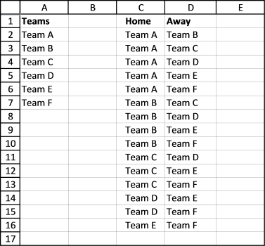
1. Basic scheduling - each team plays once against another team
The following VBA code creates a schedule where each team plays once against another team.
'Name
Function roundrobin(rng As Range)
'Get Digital Help https://www.get-digital-help.com/round-robin-tournament/

'Dimension variables and declare data types
Dim tmp() As Variant, k As Long
Dim i As Long, j As Long

'ReDimension array variable tmp
ReDim tmp(1 To (rng.Cells.Count / 2) * (rng.Cells.Count - 1), 1 To 2)

'Save 1 to variable k
k = 1

'Schedule everyone with everyone
'For ... Next statement
'Go from 1 to the number of cells in range variable rng
For i = 1 To rng.Cells.Count

'Go from i + 1 to the number of cells in range variable rng
For j = i + 1 To rng.Cells.Count

'Save value stored in worksheet based on variable i to array variable tmp based on variable k
tmp(k, 1) = rng.Cells(i)

'Save value stored in worksheet based on variable j to array variable tmp based on variable k
tmp(k, 2) = rng.Cells(j)

'Add 1 to the number stored in variable k and save to variable k
k = k + 1

'Continue with next number stored in variable j
Next j

'Continue with next number stored in variable i
Next i

'Return array to worksheet
roundrobin = tmp

End Function
As you can see it is not very complicated and the first team has home matches all the time. But if home and away doesn't matter this could useful.
Another bad thing with this custom function is that it doesn't split the schedule into rounds. A team can't play twice in the same round, obviously.
Also if you want the schedule to be somewhat random, this custom function is not for you.
The next custom function takes care of these three issues.
2. Round-robin tournament - distributes home and away rounds evenly
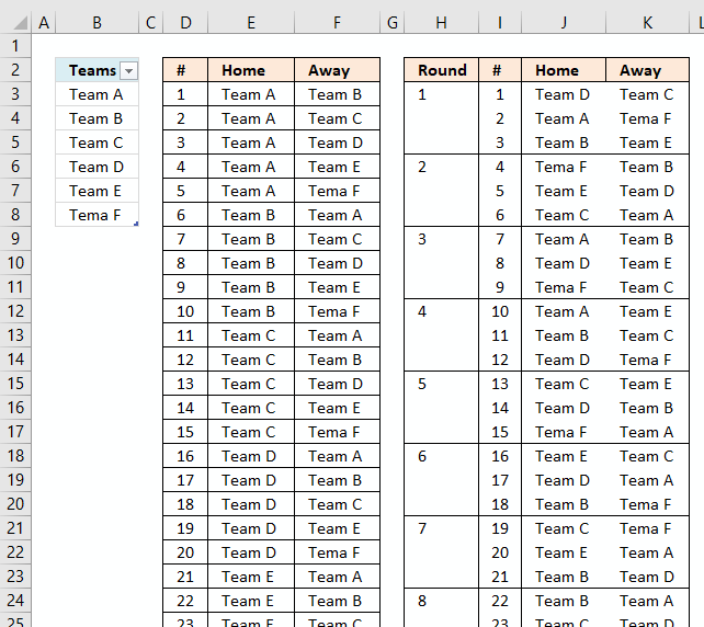
This custom function creates a round-robin tournament. It tries to distribute home and away rounds evenly and teams are randomly placed in the schedule.
'Name User Defined Function and specify parameters
Function RoundRobin2(rng As Range)
'This custom function adds a team automatically if the number of teams is uneven.
'Get Digital Help https://www.get-digital-help.com/round-robin-tournament/

'Dimension variables and declare data types
Dim tmp() As Variant, k As Long, l As Integer
Dim i As Long, j As Long, a As Long, r As Long
Dim rngA As Variant, Stemp As Variant, Val As Long
Dim res, rngB() As Variant, result As String

'Transfer cell values to an array
rngA = rng.Value

'Check if the number of teams are even
If rng.Cells.Count Mod 2 = 0 Then

'Save cell values in variable rng to variable rngB
rngB = rng.Value

'Save 0 (zero) to l
l = 0

'Continue here if the number of teams are not even
Else

'Redimension array variable rngB
ReDim rngB(1 To UBound(rngA) + 1, 1 To 1)

'For... Next statement
For i = 1 To UBound(rngA)

'Save value in array variable rngA to array variable rngB
rngB(i, 1) = rngA(i, 1)
Next i

'Save character - to the last container in array variable rngB
rngB(UBound(rngB, 1), 1) = "-"

'Save 1 to variable l
l = 1
End If

'Redimension array variable tmp
ReDim tmp(1 To ((rng.Cells.Count + l) / 2) * (rng.Cells.Count + l - 1), 1 To 3)

'Randomize array
rngB = RandomizeArray1(rngB)

Val = (UBound(rngB, 1) / 2)

'Build schedule
For i = 2 To UBound(rngB, 1)

'Save 1 to variable a
a = 1

'For ... Next statement
'Go from 1 to half of the number of rows in array variable rng2
For r = 1 To (UBound(rngB, 1) / 2)

tmp(r + Val * (i - 2), 1) = i - 1
If (i - 1) Mod 2 = 1 Then
tmp(r + Val * (i - 2), 2) = rngB(a, 1)
tmp(r + Val * (i - 2), 3) = rngB(UBound(rngB, 1) - a + 1, 1)
Else
tmp(r + Val * (i - 2), 2) = rngB(UBound(rngB, 1) - a + 1, 1)
tmp(r + Val * (i - 2), 3) = rngB(a, 1)
End If
a = a + 1
Next r

'switch places for all values except the first one
For j = 2 To UBound(rngB, 1) - 1
Stemp = rngB(j, 1)
rngB(j, 1) = rngB(j + 1, 1)
rngB(j + 1, 1) = Stemp
Next j
Next i

'Return values in array variable tmp to worksheet
RoundRobin2 = tmp

End Function
This User Defined Function creates a random schedule split into rounds, home and away are also somewhat evenly distributed through the schedule.
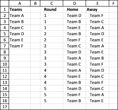
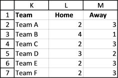
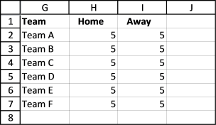
This table shows you how many times 6 teams play home and away for the entire tournament.
3. Double round-robin tournament - User Defined Function
To make sure every team has as many home as away rounds competitors play each other twice. It is a "double" round-robin tournament. The way it works is all play all twice, once home and once away.
'Name User Defined Function and specify parameters
Function doubleroundrobin(rng As Range)
'Get Digital Help https://www.get-digital-help.com/round-robin-tournament/

'Dimension variables and declare data types
Dim tmp() As Variant, k As Long, l As Integer
Dim i As Long, j As Long, a As Long, r As Long
Dim rngA As Variant, Stemp As Variant, Val As Long
Dim res, rngB() As Variant, result As String, cc As Long

'Transfer values to an array
rngA = rng.Value

'Check if the number of teams are even
If rng.Cells.Count Mod 2 = 0 Then
rngB = rng.Value
l = 0
Else
ReDim rngB(1 To UBound(rngA) + 1, 1 To 1)
For i = 1 To UBound(rngA)
rngB(i, 1) = rngA(i, 1)
Next i
rngB(UBound(rngB, 1), 1) = "-"
l = 1
End If

cc = ((rng.Cells.Count + l) / 2) * (rng.Cells.Count + l - 1)

'Redimension array variable tmp
ReDim tmp(1 To cc * 2, 1 To 3)

'Randomize array
rngB = RandomizeArray1(rngB)

'Save half of the number of rows in array variable rngB to variable Val
Val = (UBound(rngB, 1) / 2)

'Build schedule
For i = 2 To UBound(rngB, 1)

a = 1
For r = 1 To (UBound(rngB, 1) / 2)
tmp(r + Val * (i - 2), 1) = i - 1
If (i - 1) Mod 2 = 1 Then
tmp(r + Val * (i - 2), 2) = rngB(a, 1)
tmp(r + Val * (i - 2), 3) = rngB(UBound(rngB, 1) - a + 1, 1)
Else
tmp(r + Val * (i - 2), 2) = rngB(UBound(rngB, 1) - a + 1, 1)
tmp(r + Val * (i - 2), 3) = rngB(a, 1)
End If
a = a + 1
Next r
For j = 2 To UBound(rngB, 1) - 1
Stemp = rngB(j, 1)
rngB(j, 1) = rngB(j + 1, 1)
rngB(j + 1, 1) = Stemp
Next j
Next i

'Copy schedule and change home to away and vice versa, this makes it a double round-robin tournament
For i = cc + 1 To cc * 2
tmp(i, 1) = UBound(rngB, 1) - 1 + tmp(i - cc, 1)
tmp(i, 2) = tmp(i - cc, 3)
tmp(i, 3) = tmp(i - cc, 2)
Next i

'Return values in array variable tmp to worksheet
doubleroundrobin = tmp

End Function
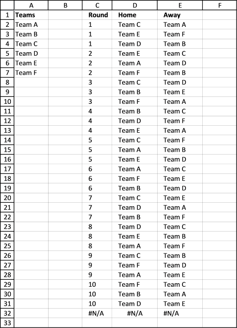
Here is a table that shows you teams play as many home as away games.
4. Macro
The macros in the workbook below allow you to create a match schedule. Go to sheet Macro and follow instructions.
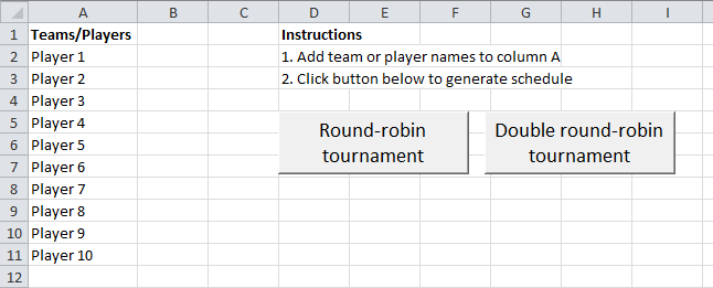
Add teams or players to column A, then press with left mouse button on the "Round-robin tournament" button or "Double round-robin tournament".
A match schedule is created on a new sheet.
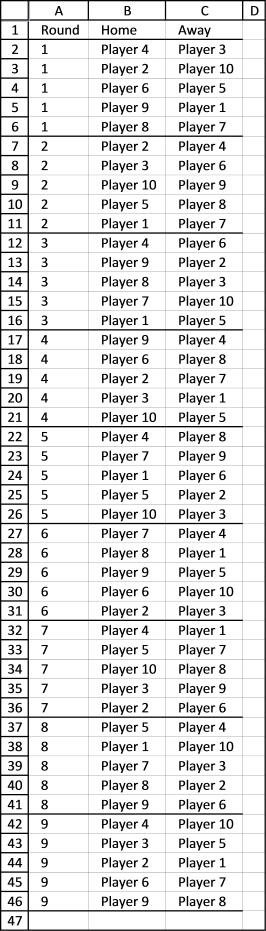
Conditional formatting separates rounds with a line, it makes the table easier to read.
Round-robin tournament
Sub rr()
'Get Digital Help, https://www.get-digital-help.com/round-robin-tournament/

Dim Lrow As Long
Dim rng As Range, tmp() As Variant
Dim ws As Worksheet
Application.ScreenUpdating = False
Lrow = Worksheets("Macro").Range("A" & Rows.Count).End(xlUp).Row
Set rng = Worksheets("Macro").Range("A2:A" & Lrow)

tmp = RoundRobin2(rng)

'Insert new sheet
Set ws = Sheets.Add

ws.Range("A1") = "Round"
ws.Range("B1") = "Home"
ws.Range("C1") = "Away"
ws.Range("A2").Resize(UBound(tmp, 1), 3) = tmp

ws.Range("A1").Resize(UBound(tmp, 1) + 1, 3).InsertIndent 1
Columns("A:C").EntireColumn.AutoFit
ws.Range("A1:C1000").Select
Selection.FormatConditions.Add Type:=xlExpression, Formula1:="=$A1<>$A2"
Selection.FormatConditions(Selection.FormatConditions.Count).SetFirstPriority
With Selection.FormatConditions(1).Borders(xlBottom)
.LineStyle = xlContinuous
.TintAndShade = 0
.Weight = xlThin
End With
Selection.FormatConditions(1).StopIfTrue = False
Application.ScreenUpdating = True
End Sub
Double round-robin tournament
Sub droundrobin()
Dim Lrow As Long
Dim rng As Range, tmp() As Variant
Dim ws As Worksheet
Application.ScreenUpdating = False
Lrow = Worksheets("Macro").Range("A" & Rows.Count).End(xlUp).Row
Set rng = Worksheets("Macro").Range("A2:A" & Lrow)

tmp = doubleroundrobin(rng)

'Insert new sheet
Set ws = Sheets.Add

ws.Range("A1") = "Round"
ws.Range("B1") = "Home"
ws.Range("C1") = "Away"
ws.Range("A2").Resize(UBound(tmp, 1), 3) = tmp

ws.Range("A1").Resize(UBound(tmp, 1) + 1, 3).InsertIndent 1
Columns("A:C").EntireColumn.AutoFit
ws.Range("A1:C1000").Select
Selection.FormatConditions.Add Type:=xlExpression, Formula1:="=$A1&<>$A2"
Selection.FormatConditions(Selection.FormatConditions.Count).SetFirstPriority
With Selection.FormatConditions(1).Borders(xlBottom)
.LineStyle = xlContinuous
.TintAndShade = 0
.Weight = xlThin
End With
Selection.FormatConditions(1).StopIfTrue = False
Application.ScreenUpdating = True
End Sub
This function moves values in an array randomly.
'Name User Defined Function
Function RandomizeArray1(Arr As Variant)

'Dimension variables and declare data types
Dim temp
Dim i As Long, j As Long, k As Long
Dim result As Variant

'For ... Next statement
For k = LBound(Arr, 1) To UBound(Arr, 1)

'Add values to variable result
result = result & Arr(k, 1) & " "

Next k

'Add new line to variable result
result = result & vbNewLine

'For ... Next statement
For i = LBound(Arr, 1) To UBound(Arr, 1)

'Generate random value
j = Application.WorksheetFunction.RandBetween(LBound(Arr, 1), UBound(Arr, 1))

'Save value in array variable Arr to temp
temp = Arr(j, 1)
Arr(j, 1) = Arr(i, 1)
Arr(i, 1) = temp
For k = LBound(Arr, 1) To UBound(Arr, 1)
result = result & Arr(k, 1) & " "
Next k
result = ""
Next i

RandomizeArray1 = Arr

End Function
5. How to use a custom function
If you want the vba code in your own workbook, do this.
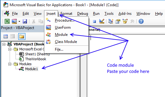
- Press Alt-F11 to open visual basic editor
- Press with left mouse button on Module on the Insert menu
- Copy and paste all custom functions above to the code module
- Exit visual basic editor (Alt+Q)
- Save your workbook as a *.xlsm file
Now you can use the custom functions. Type your teams in a column. Select a blank cell range, 3 columns wide and many rows, you can extend this later if not all rounds show up.
Type =doubleroundrobin(cell_ref_to_your_teams), press and hold CTRL + Shift. Press Enter. Release all keys.
7. True round-robin tournament
Mark G asks in Create a random playlist in excel:
Can this example be modified to create a true round-robin draw?
i.e. using a 6 team scenario, for any round there will be three games/matches, but obviously, Team A could not compete against say Team B and Team C during that round as can occur using the above formula.
Answer:
This example is based on a double round-robin in which every team plays all others in its league once at home and once away randomly.
The picture above shows two playlists, the random playlist is the right one. Each round is divided using conditional formatting.
The worksheet is dynamic meaning you can have more or less teams and the worksheet will automatically generate a random playlist for you.
You can get the workbook at the end of this article.
How to use this workbook
The first playlist table is not random, it simply lists all possible matches for the entered team names. The second list is random.
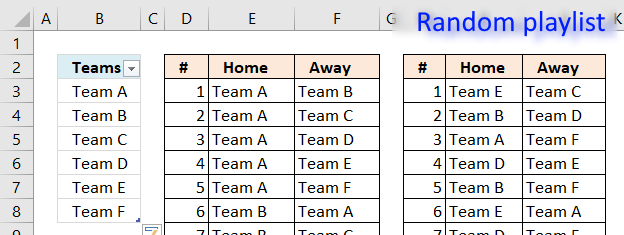
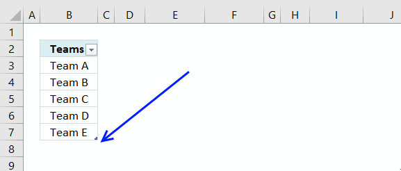
You type the team names in column B in the Excel defined Table. It automatically expands when new values are entered, you don't need to adjust any formulas or cell references.
Add team names
Simply type the next Team name in the first empty cell below the table.
Delete team names
To delete a name in the Excel defined table you need to select the cells you want to delete.
Then press with right mouse button on on the selected range.
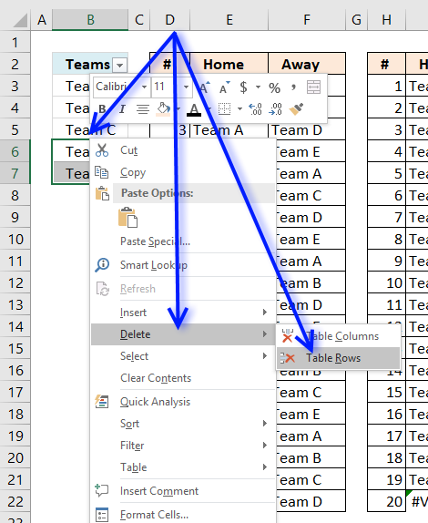
Press with mouse on "Delete" and then press with left mouse button on "Table Rows".
If you accidentally press with left mouse button on "Table Columns", don't freak out. Simply press CTRL + z to undo.
Edit team names
You can edit the existing team names as well, the formulas are dynamic and return the correct names in the playlist instantly.
Generate the tournament playlist
There is a button to the right of the playlists.
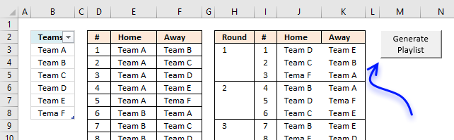
Press with left mouse button on the button to automatically generate a new random playlist determined by the number of teams you have entered in column B.
When you have a playlist you are happy with copy it and paste it to a new worksheet.
What does this workbook contain to make this possible?
Formula in cell D3 and below:
Formula in cell E3 and below:
Formula in cell F3 and below:
Formula in cell H3 and below:
Formula in cell I3 and below:
Formula in cell J3 and below:
Formula in cell K3 and below:
Hidden formula in cell L3 and below:
Hidden formula in cell M2:
Hidden formula in cell M3 and cells below:
VBA Macro
The random playlist sometimes returns error values, the following code verifies that no errors occur.
Sub GeneratePlayList()
Application.ScreenUpdating = False
Do
Calculate
DoEvents
Loop While Worksheets("Sheet1").Range("M2") <> 0
Application.ScreenUpdating = True
End Sub
8. Create a random playlist
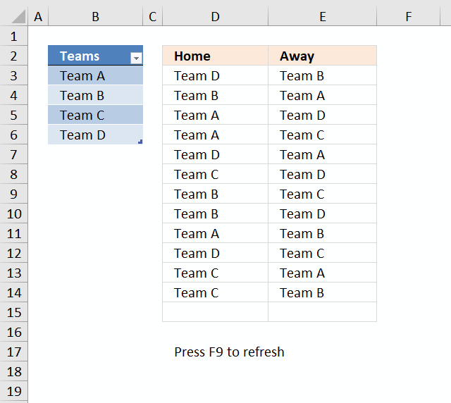
This article describes how to create a random playlist based on a given number of teams using an array formula. Column A contains four teams. Each team plays matches both "Home" against all remaining teams and "Away" against all remaining teams.
The teams are entered in an Excel defined table, this allows you to add or delete teams without the need to adjust cell references in the formulas. The calculation also takes into account the number of teams so the only thing for you to do is to extend the formulas down as far as needed.
Example:
Team A plays "Home" against Team B, Team C and Team D.
Team A- Team B
Team A - Team C
Team A - Team D
Team A plays also "Away" against Team B, Team C and Team D.
Team B - Team A
Team C - Team A
Team D - Team A
Column C and Column D contain a random playlist. Press F9 to refresh.
Array formula in D3:
To enter an array formula, type the formula in a cell then press and hold CTRL + SHIFT simultaneously, now press Enter once. Release all keys.
The formula bar now shows the formula with a beginning and ending curly bracket telling you that you entered the formula successfully. Don't enter the curly brackets yourself.
If column A contains five teams, change ROW($1:$4) to ROW($1:$5) and bolded 3's to 4 in the above formula. Don't forget to adjust cell references.
Array formula i E3:
If column A contains five teams, change ROW($1:$4) to ROW($1:$5) and bolded 3's to 4 in the above formula. Don't forget to adjust cell references accordingly as well.
Explaining formula in cell D3
There is an explanation to this formula in this post: Team generator
Explaining formula in cell E3
Step 1 - Count previous teams in cells above
The COUNTIF function counts values based on a condition or criteria, the first argument contains an expanding cell reference, it grows when the cell is copied to cells below. This makes the formula aware of values displayed in cells above. 0 (zero) indicates values that not yet have been displayed.
COUNTIF($E$2:E2,Table1[Teams])
becomes
COUNTIF($E$2:E2,$B$3:$B$6)
becomes
COUNTIF("Away",{"Team A"; "Team B"; "Team C"; "Team D"})
and returns {0;0;0;0}.
Step 2 - Count non-empty cells
The COUNTA function counts cells that are not empty based on a given cell range.
COUNTA(Table1[Teams])-1
becomes
COUNTA($B$3:$B$6)-1
becomes
COUNTA({"Team A"; "Team B"; "Team C"; "Team D"})-1
becomes
4-1
and returns 3.
Step 3 - Compare array with the number of teams - 1
COUNTIF($E$2:E2, Table1[Teams])<(COUNTA(Table1[Teams])-1)
becomes
{0;0;0;0}<3
and returns
{TRUE; TRUE; TRUE; TRUE}
Step 4 - Prevent home team from being selected again
COUNTIF(D3,Table1[Teams])=0
becomes
COUNTIF("Team D",{"Team A"; "Team B"; "Team C"; "Team D"})=0
becomes
{0;0;0;1}=0
and returns
{TRUE; TRUE; TRUE; FALSE}
Step 5 - Prevent duplicate matches
This step makes sure that the same team is not being in the list more than once against a given Home team. There are two expanding cell references that grow when the cell is copied to cells below.
ISERROR(MATCH(Table1[Teams], IF(D3=$D$2:D2, $E$2:E2, ""), 0))
becomes
ISERROR(MATCH(Table1[Teams], IF("Team D"="Home", "Away", ""), 0))
becomes
ISERROR(MATCH(Table1[Teams], "", 0))
becomes
ISERROR(MATCH({"Team A"; "Team B"; "Team C"; "Team D"}, "", 0))
becomes
ISERROR({#VALUE!; #VALUE!; #VALUE!; #VALUE!})
and returns
{TRUE; TRUE; TRUE; TRUE}
Step 6 - Multiply arrays
This step applies and logic between the arrays meaning all conditions must be TRUE. TRUE * TRUE = TRUE, TRUE * FALSE = FALSE and FALSE * FALSE = FALSE. TRUE is 1 and FALSE is 0 (zero).
(COUNTIF($E$2:E2,Table1[Teams])<(COUNTA(Table1[Teams])-1))*(COUNTIF(D3,Table1[Teams])=0)*(ISERROR(MATCH(Table1[Teams],IF(D3=$D$2:D2,$E$2:E2,""),0)))*ROW($1:$4)
becomes
{TRUE; TRUE; TRUE; TRUE}* {TRUE; TRUE; TRUE; FALSE}* {TRUE; TRUE; TRUE; TRUE}* ROW($1:$4)
becomes
{1; 1; 1; 0}* ROW($1:$4)
The array is the multiplied to a sequence of row numbers.
{1; 1; 1; 0}* ROW($1:$4)
becomes
{1; 1; 1; 0}* {1; 2; 3; 4}
and returns {1; 2; 3; 0}
Step 6 - Extract random row number
The LARGE function returns the k-th largest number, LARGE( array , k). The second argument k is a random number from 1 to n.
LARGE((COUNTIF($D$2:D2, Table1[Teams])<(COUNTA(Table1[Teams])-1))*ROW($1:$4), RANDBETWEEN(1, SUMPRODUCT(--((ISERROR(MATCH(Table1[Teams], IF(D3=$D$2:D2, $E$2:E2, ""), 0)))*(COUNTIF($E$2:E2, Table1[Teams])<(COUNTA(Table1[Teams])-1))*(COUNTIF(D3, Table1[Teams])=0))))))
becomes
LARGE({1; 2; 3; 0}, RANDBETWEEN(1, SUMPRODUCT(--((ISERROR(MATCH(Table1[Teams], IF(D3=$D$2:D2, $E$2:E2, ""), 0)))*(COUNTIF($E$2:E2, Table1[Teams])<(COUNTA(Table1[Teams])-1))*(COUNTIF(D3, Table1[Teams])=0)))))
The RANDBETWEEN function returns a random number based on the two arguments.
LARGE({1; 2; 3; 0}, RANDBETWEEN(1, SUMPRODUCT(--({TRUE; TRUE; TRUE; TRUE}*(COUNTIF($E$2:E2, Table1[Teams])<(COUNTA(Table1[Teams])-1))*(COUNTIF(D3, Table1[Teams])=0)))))
becomes
LARGE({1; 2; 3; 0}, RANDBETWEEN(1, SUMPRODUCT(--({TRUE; TRUE; TRUE; TRUE}*{TRUE; TRUE; TRUE; TRUE}*(COUNTIF(D3, Table1[Teams])=0)))))
becomes
LARGE({1; 2; 3; 0}, RANDBETWEEN(1, SUMPRODUCT(--({TRUE; TRUE; TRUE; TRUE}*{TRUE; TRUE; TRUE; TRUE}*{TRUE; TRUE; TRUE; FALSE}))))
becomes
LARGE({1; 2; 3; 0}, RANDBETWEEN(1, SUMPRODUCT({1; 1; 1; 0})))
becomes
LARGE({1; 2; 3; 0}, RANDBETWEEN(1, 3))
becomes
LARGE({1; 2; 3; 0}, 2)
and returns 2. This is a random value between 1 and 3.
Step 7 - Return value
The INDEX function returns a value based on a cell reference and column/row numbers.
INDEX(Table1[Teams], LARGE((COUNTIF($E$2:E2, Table1[Teams])<(COUNTA(Table1[Teams])-1))*(COUNTIF(D3, Table1[Teams])=0)*(ISERROR(MATCH(Table1[Teams], IF(D3=$D$2:D2, $E$2:E2, ""), 0)))*ROW($A$1:INDEX($A$1:$A$1000, COUNTA(Table1[Teams]))), RANDBETWEEN(1, SUMPRODUCT(--((ISERROR(MATCH(Table1[Teams], IF(D3=$D$2:D2, $E$2:E2, ""), 0)))*(COUNTIF($E$2:E2, Table1[Teams])<(COUNTA(Table1[Teams])-1))*(COUNTIF(D3, Table1[Teams])=0))))))
becomes
INDEX(Table1[Teams], 2)
and returns "Team B" in cell D3.
Random category
Table of Contents Team Generator Dynamic team generator How to build a Team Generator - different number of people per […]
Tournament category
More than 1300 Excel formulasExcel categories
9 Responses to “How to generate a round-robin tournament”
Leave a Reply
How to comment
How to add a formula to your comment
<code>Insert your formula here.</code>
Convert less than and larger than signs
Use html character entities instead of less than and larger than signs.
< becomes < and > becomes >
How to add VBA code to your comment
[vb 1="vbnet" language=","]
Put your VBA code here.
[/vb]
How to add a picture to your comment:
Upload picture to postimage.org or imgur
Paste image link to your comment.
Oscar
Thank you for this work. This is exactly what I need for a small / local table football league we have just started. Thank you very much.
Guy
will try this later
Hi Oscar,
I found this during my searches for finding a "perfect" scheduler of round-robun tournament, and i have to say this is closely to perfection.
The only thing I can remark, is that system home-away is not so accurate, even in your example, Player 3 plays 2 times away (round 5 and 6) and Player 10 2 times (round 8 and 9), and exemples still there are, with Player 7...
Maybe a round robin tournament could not be perfect, regarding home-away matches ?
Awesome!!
No logro abrir el archivo me marca como archivo dañado, no se si tenga algun codigo de acceso o algo así
Hello Oscar, your code for creating Round Robin Tournaments works great and obviously it's extremely flexible. I am using mine for a 16 Team Golf Schedule that has a Shotgun Start. I was hoping to include what Hole each of the competitions would start on (1-8) in the schedule. Unfortunately, most generators don't evenly balance the Team and the starting hole. Example: Team 1 might start on the 1st Hole every week instead of an even spread over all the holes throughout the year. Do you know of such a code?
Thanks for what you have given us so far...Mike
Oscar,
i did a tryout for a double round-robin tournament with 10 teams.
But when i release the keys I get 10 rows after round 9 with only zeros in it an then he restarts with round 10 to round 18.
Screenshot under link https://postimg.cc/dLtqVwTS
Luc,
Hi Oscar,
This is exactly what I am looking for. In the marco, what variable do I update if I want to #n round-robin rather than just Double round-robin.
Is there a way I can add category as well, so i will generate the schedule by category?
Example:
Teams/Players Sport
Team1 Basketball
Team2 Baseball
Team3 Basketball
Team4 Baseball
La generacion de un fixture round robin con la aplicacion excell que muestran presenta varias imprecisiones: no respeta ranking de netrada, no mantiene igual cantidad de veces local vs visita etc