How to use the COUNTA function
What is the COUNTA function?
The COUNTA function counts the non-empty or non-blank cells in a cell reference.
Table of Contents
- Syntax
- Arguments
- Example
- Count non-empty values in an array
- Count non-empty values based on a condition
- Count non-empty values based on a list
- Count non-empty values in a string
- Count non-empty cells in multiple cell ranges
- Count non-empty cells per row
- Sort rows based on the number of non-empty cells
- Count non-empty cells per column
- Sort columns based on the number of non-empty cells
- Function not working
- Get Excel *.xlsx file
1. Syntax
COUNTA(value1, [value2], ...)
2. Arguments
| value1 | Required. A cell reference to a range for which you want to count not empty values. |
| [value2] | Optional. Up to 254 additional arguments like the one above. |
The COUNTA function counts errors as not empty.
3. Example
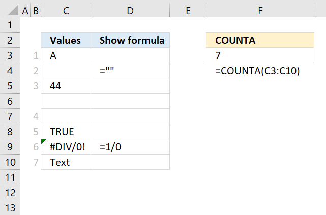
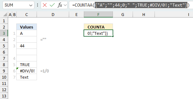
The picture above demonstrates the COUNTA function which counts non-empty or non-blank cells. Cell range C3:C10 contains data and some formulas, cell range D3:D10 shows the formulas in the corresponding cells on the same row. For example, cell D3 shows this formula: ="". It means that cell C3 contains this formula. If the cell in D3:D10 is empty the corresponding cell in C3:C10 contains a non-formula value.
This setup is to show how the COUNTA function handles text, numbers, boolean values, formulas and blank cells. The gray numbers in column B shows which values are evaluated as non-blank cells and as you can see only cell C6 is truly blank.
- Cell C3 contains a text value "A", this is a non-blank value hence the gray count in cell B3.
- Cell C4 contains a formula that returns nothing (blank), however, the COUNTA function considers this as a non-empty cell probably because it contains a formula.
- Cell C5 contains number 44. This is a non-empty value.
- Cell C6 is a blank empty cell. The COUNTA function doesnt count this cell, it counts only non-empty cells.
- Cell C7 contains a space character, the cell looks empty but is not. This cell is counted.
- Cell C8 contains a bollean value TRUE. This cell is counted.
- Cell C9 contains an Excel error. This cell is counted.
- Cell C10 contains a text string "Text". This cell is counted.
Formula in cell F3:
Cell range C3:C10 contains 8 cells, however, only one cell is truly empty. The COUNTA function returns 7 (8-1). I hope this demonstration shows how the COUNTA function handles different cells based on the content.
4. Count non-empty values in an array

This demonstrates that if you hardcode values in an COUNTA function, make sure you don't use empty values. The array containing hard-coded values are: {"A";;"";44;0;" ";TRUE;#DIV/0!;"Text"}. The semicolon is a delimiting character that separates values by row. If nothing exist between two semicolon like this: ;; then Excel shows an ugly dialog box telling you there is a typo with this formula.
This means that you can't use arrays with empty values, in other words, the COUNTA function is worthless for counting non-empty values because you can't have empty values in an hard-coded array.
Formula in cell B3:
The formula above does not work, however, the formula below works.

The COUNTA function works if all containers in the array are non-empty, which makes this function useless for hard-coded arrays.
Formula in cell B3:
An empty container like this "" is not considered empty which is surprising. The following formula counts non empty values in a hard-coded array.
Explaining formula
Step 1 - Replace errors with a text value
The IFERROR function catches most errors in Excel formulas.
IFERROR(value, value_if_error)
IFERROR({"A";"";44;0;" ";TRUE;#DIV/0!;"Text"},"A")
returns
{"A"; ""; 44; 0; " "; TRUE; "A"; "Text"}
Step 2 - Check if not empty
The less than and the larger than characters combined lets you test if a value is not equal to another value. The result is either TRUE or FALSE.
(IFERROR({"A";"";44;0;" ";TRUE;#DIV/0!;"Text"},"A")<>""
becomes
{"A"; ""; 44; 0; " "; TRUE; "A"; "Text"}<>""
and returns
{TRUE; FALSE; TRUE; TRUE; TRUE; TRUE; TRUE; TRUE}.
Step 3 - Convert boolean values to the numerical equivalents
This step is need in order to calculate a sum, the SUMPRODUCT function in the next step can't work with boolean values, however, their numerical equivalents work fine.
(IFERROR({"A";"";44;0;" ";TRUE;#DIV/0!;"Text"},"A")<>"")*1
becomes
{TRUE; FALSE; TRUE; TRUE; TRUE; TRUE; TRUE; TRUE}*1
returns
{1; 0; 1; 1; 1; 1; 1; 1}.
Step 4 - Calculate a total
The SUMPRODUCT function calculates the product of corresponding values and then returns the sum of each multiplication.
SUMPRODUCT(array1, [array2], ...)
SUMPRODUCT((IFERROR({"A";"";44;0;" ";TRUE;#DIV/0!;"Text"},"A")<>"")*1)
becomes
SUMPRODUCT({1; 0; 1; 1; 1; 1; 1; 1})
and returns 8.
5. Count non-empty values based on a condition

This example demonstrates how to count non-blank cells based on a condition applied to an adjacent column. The image above shows the condition in cell E3, cell range B3:B11 contains the values and the corresponding values in cell range C3:C11 contain numbers and some blank cells.
Formula in cell F3:
The formula in cell F3 matches the condition to B3:B11 and the corresponding matching cells are C5, C10 and C11. Cells C5 and C11 contain numbers, however, cell C10 is blank. The formula returns 2, there are two nonempty cells based on the given condition.
Explaining formula
The "Evaluate" tool on tab "Formula" on the ribbon lets you examine formulas in greater detail. It lets you see the calculation step by step making it much easier to understand and troubleshoot formulas.
Step 1 - Logical expression
The equal sign lets you compare value to value, it can also be used to compare a single value to multiple different values. The result is a boolean value, it is either TRUE or FALSE.
B3:B11=E3
becomes
{"Pen"; "Pencil"; "Clip"; "Pen"; "Clip"; "Pencil"; "Pen"; "Clip"; "Clip"}="Clip"
and returns
{FALSE; FALSE; TRUE; FALSE; TRUE; FALSE; FALSE; TRUE; TRUE}.
Step 2 - Check if not empty (non-empty)
The less than sign and the larger than sign combined lets you check if a value is NOT equal to another value. We are comparing nothing in this example to multiple cells, there is nothing between the double quotes "". The result is a boolean value, it is either TRUE or FALSE or in this case an array containing boolean values.
C3:C11<>""
becomes
{""; 7; 45; 31; ""; 37; 98; ""; 6}<>""
and returns
{FALSE; TRUE; TRUE; TRUE; FALSE; TRUE; TRUE; FALSE; TRUE}
Step 3 - Evaluate IF function
The IF function returns one value if the logical test is TRUE and another value if the logical test is FALSE.
IF(logical_test, [value_if_true], [value_if_false])
IF(B3:B11=E3,C3:C11<>"",0)
becomes
IF({FALSE; FALSE; TRUE; FALSE; TRUE; FALSE; FALSE; TRUE; TRUE},C3:C11<>"",0)
becomes
IF({FALSE; FALSE; TRUE; FALSE; TRUE; FALSE; FALSE; TRUE; TRUE},{FALSE; TRUE; TRUE; TRUE; FALSE; TRUE; TRUE; FALSE; TRUE},0)
and returns
{0; 0; TRUE; 0; FALSE; 0; 0; FALSE; TRUE}
Step 4 - Convert boolean values
The SUM function can't calculate a total using boolean values, we need to convert the boolean values to their numerical equivalents.
TRUE - 1
FALSE - 0 (zero)
The asterisk lets you multiply numbers and boolean values in an Excel formula.
IF(B3:B11=E3,C3:C11<>"",0)*1
becomes
{0; 0; TRUE; 0; FALSE; 0; 0; FALSE; TRUE}*1
and returns
{0; 0; 1; 0; 0; 0; 0; 0; 1}. All values in the array are now either 1 or 0 (zero).
Step 5 - Calculate a total
The SUM function adds values and returns a total.
SUM(number1, [number2], ...)
SUM(IF(B3:B11=E3,C3:C11<>"",0)*1)
becomes
SUM({0; 0; 1; 0; 0; 0; 0; 0; 1})
and returns 2.
6. Count non-empty values based on a list

This example shows how to count non-empty cells based on multiple conditions, the conditions are specified in cell E3:E4. The formula counts non-empty cells if they are on the same row as at least one of the conditions.
Formula in cell F3:
The image above shows the criteria in cell E3 and E4, the matching cells in cell range B3:B11 are B3, B5, B6, B7, B9, B10 and B11. The corresponding cells on the same row in column C have four non-empty cells. They are C5, C6, C9, and C11.
Explaining formula
Step 1 - Which values equal any item in the list
The COUNTIF function counts the number of cells that meet a given condition.
COUNTIF(range, criteria)
COUNTIF(E3:E4, B3:B11)
becomes
COUNTIF({"Clip"; "Pen"}, {"Pen"; "Pencil"; "Clip"; "Pen"; "Clip"; "Pencil"; "Pen"; "Clip"; "Clip"})
and returns
{1; 0; 1; 1; 1; 0; 1; 1; 1}.
Step 2 - Check if not empty (non-empty)
The less than sign and the larger than sign combined lets you check if a value is NOT equal to another value. This example checks if the values are empty.
C3:C11<>""
becomes
{""; 7; 45; 31; ""; 37; 98; ""; 6}<>""
and returns
{FALSE; TRUE; TRUE; TRUE; FALSE; TRUE; TRUE; FALSE; TRUE}.
Step 3 - Evaluate IF function
The IF function returns one value if the logical test is TRUE and another value if the logical test is FALSE.
IF(logical_test, [value_if_true], [value_if_false])
IF(COUNTIF(E3:E4, B3:B11), C3:C11<>"", 0)
becomes
IF({1; 0; 1; 1; 1; 0; 1; 1; 1}, {FALSE; TRUE; TRUE; TRUE; FALSE; TRUE; TRUE; FALSE; TRUE}, 0)
and returns
{FALSE; 0; TRUE; TRUE; FALSE; 0; TRUE; FALSE; TRUE}.
Step 4 - Convert boolean values
The SUM function can't calculate a total using boolean values, we need to convert the boolean values to their numerical equivalents.
TRUE - 1
FALSE - 0 (zero)
The asterisk lets you multiply numbers and boolean values in an Excel formula.
IF(B3:B11=E3,C3:C11<>"",0)*1
becomes
{FALSE; 0; TRUE; TRUE; FALSE; 0; TRUE; FALSE; TRUE}*1
and returns
{0; 0; 1; 1; 0; 0; 1; 0; 1}.
Step 5 - Calculate a total
The SUM function adds values and returns a total.
SUM(number1, [number2], ...)
SUM(IF(B3:B11=E3,C3:C11<>"",0)*1)
becomes
SUM({0; 0; 1; 1; 0; 0; 1; 0; 1})
and returns 4.
7. Count non-empty values in a string

This example demonstrates how to count non-blank values in an array created from a string of delimited values using the TEXTSPLIT function. The image above shows a string in cell B3 containing the delimiting value |.
Excel 365 dynamic array formula in cell D3:
The formula in cell D3 splits the string in cell B3 based on the delimiting character |.
|7|45|31||37|98||6 returns the following values: 7, 45, 31, "",37,98,"", and 6. It is now clear that the string contains two empty array containers "".
Explaining formula
Step 1 - Split values
The TEXTSPLIT function lets you split a string into an array across columns and rows based on delimiting characters.
TEXTSPLIT(Input_Text, col_delimiter, [row_delimiter], [Ignore_Empty])
TEXTSPLIT(C3,";")
becomes
TEXTSPLIT("|7|45|31||37|98||6","|")
and returns
{"", "7", "45", "31", "", "37", "98", "", "6"}.
Step 2 - Check if values in array are not empty
The less than sign and the larger than sign combined lets you check if a value is NOT equal to another value. This example checks if the values are empty.
TEXTSPLIT(C3,";")<>""
becomes
{"", "7", "45", "31", "", "37", "98", "", "6"}<>""
and returns
{FALSE, TRUE, TRUE, TRUE, FALSE, TRUE, TRUE, FALSE, TRUE}.
Step 3 - Convert boolean values
The SUM function can't calculate a total using boolean values, we need to convert the boolean values to their numerical equivalents.
TRUE - 1
FALSE - 0 (zero)
The asterisk lets you multiply numbers and boolean values in an Excel formula.
(TEXTSPLIT(C3,";")<>"")*1
becomes
{FALSE, TRUE, TRUE, TRUE, FALSE, TRUE, TRUE, FALSE, TRUE}*1
and returns
{0, 1, 1, 1, 0, 1, 1, 0, 1}
Step 4 - Add numbers and return a total
The SUM function adds values and returns a total.
SUM(number1, [number2], ...)
SUM((TEXTSPLIT(C3,";")<>"")*1)
becomes SUM({0, 1, 1, 1, 0, 1, 1, 0, 1})
and returns 6.
8. Count non-empty cells in multiple cell ranges

This example demonstrates a formula that counts non-empty cells in multiple cell ranges. The new Excel 365 array functions make this easy and straightforward.
Formula in cell B12:
The image above shows three nonadjacent cell ranges B3:B9, D3:D9, and F3:F9. The cell ranges don't need to be the same size vertically or horizontally, though they are in this example. The cell ranges contain values and some random blank cells, the dynamic array formula in cell B12 counts non-blank cells in all three cell ranges combined.
Cell range B3:B9 contains 6 non-empty cells, D3:D9 contains 5 non-empty cells, and F3:F9 also contains 5 non-empty cells. The total number of non-empty cells are 6 + 5 + 5 = 16
Explaining formula
Step 1 - Join arrays
The VSTACK function combines cell ranges or arrays, it joins data to the first blank cell at the bottom of a cell range or array.
VSTACK(array1,[array2],...)
VSTACK(B3:B9, D3:D9, F3:F9)
becomes
VSTACK({7;"";82;43;25;10;21},{73;13;93;"";"";65;91},{"";11;97;61;4;45;""})
and returns
{7; ""; 82; 43; 25; 1""; 21; 73; 13; 93; ""; ""; 65; 91; ""; 11; 97; 61; 4; 45; ""}.
Step 2 - Check if not empty
The less than sign and the larger than sign combined lets you check if a value is NOT equal to another value. This example checks if the values are empty.
VSTACK(B3:B9,D3:D9,F3:F9)<>""
becomes
{7; ""; 82; 43; 25; 1""; 21; 73; 13; 93; ""; ""; 65; 91; ""; 11; 97; 61; 4; 45; ""}<>""
and returns
{TRUE; FALSE; TRUE; ... ; FALSE}.
Step 3 - Convert boolean values to numbers
The SUM function can't calculate a total using boolean values, we need to convert the boolean values to their numerical equivalents.
TRUE - 1
FALSE - 0 (zero)
The asterisk lets you multiply numbers and boolean values in an Excel formula.
(VSTACK(B3:B9,D3:D9,F3:F9)<>"")*1
becomes
{TRUE; FALSE; TRUE; ... ; FALSE}*1
and returns
{1; 0; 1; 1; 1; 1; 1; 1; 1; 1; 0; 0; 1; 1; 0; 1; 1; 1; 1; 1; 0}.
Step 4 - Calculate a total
SUM((VSTACK(B3:B9,D3:D9,F3:F9)<>"")*1)
becomes
SUM({1; 0; 1; 1; 1; 1; 1; 1; 1; 1; 0; 0; 1; 1; 0; 1; 1; 1; 1; 1; 0})
and returns 16.
9. Count non-empty cells per row

The image above shows an Excel 365 dynamic array formula that returns an array of numbers representing the number of non-empty cells per row. The position in the array corresponds to the row in cell range B3:E9.
The dynamic array formula in cell G3 spills values to cell G3 and cells below as far as needed. A #SPILL! error means that at least one of the destination cells is not empty. Make sure the cells are empty so the formula can distribute the array values to a cell each.
Excel 365 formula in cell G3:
Cell range B3:E3 contains three non-empty cells and one empty cell. Cell range B4:E4 contains two non-empty cells and two empty cells.
Cell range B5:E5 also contains two non-empty cells and two empty cells, this is also true for cell range B6:E6.
Cell range B7:E7 contains four non-empty cells and 0 (zero) empty cells. Cell range B8:E8 contains two non empty cells and two empty cells. This is also true for cell range B9:E9.
Explaining formula
Step 1 - Count nonempty cells
The COUNTA function counts the non-empty or non-blank cells in a cell range.
Function syntax: COUNTA(value1, [value2], ...)
COUNTA(a)
Step 2 - Build the LAMBDA function
The LAMBDA function build custom functions without VBA, macros or javascript.
Function syntax: LAMBDA([parameter1, parameter2, …,] calculation)
LAMBDA(a,COUNTA(a))
Step 3 - Count nonempty cells per row
The BYROW function puts values from an array into a LAMBDA function row-wise.
Function syntax: BYROW(array, lambda(array, calculation))
BYROW(B3:E9,LAMBDA(a,COUNTA(a)))
10. Sort rows based on the number of non-empty cells

Excel 365 dynamic array formula in cell G3:
Explaining formula
This formula works just like the example in section 9, but it also sorts rows based on the count of nonempty cells.
The SORTBY function sorts a cell range or array based on values in a corresponding range or array.
Function syntax: SORTBY(array, by_array1, [sort_order1], [by_array2, sort_order2],…)
11. Count non-empty cells per column

The image above shows an Excel 365 dynamic array formula that returns an array of numbers representing the total number of non-e,pty cells per column.
Cell range B3:E9 contains empty cells and non-empty cells. The following formula returns an array in B11 that spills values to the right as far as needed.
Excel 365 formula in cell B11:
The formula counts the number of nonempty cells per column, and the position in the array corresponds to the column in cell range B3:E9.
Cell range B3:B9 contains one empty cell and 6 non-empty cells. Cell range C3:C9 contains four empty cells and three non-empty cells.
Cell range D3:D9 contains five non-empty cells and two empty cells. Cell range E3:E9 contains three non-empty cells and four empty cells.
Explaining formula
Step 1 - Count nonempty cells
The COUNTA function counts the non-empty or non-blank cells in a cell range.
Function syntax: COUNTA(value1, [value2], ...)
COUNTA(a)
Step 2 - Build the LAMBDA function
The LAMBDA function build custom functions without VBA, macros or javascript.
Function syntax: LAMBDA([parameter1, parameter2, …,] calculation)
LAMBDA(a,COUNTA(a))
Step 3 - Count nonempty cells per column
The BYCOL function passes all values in a column based on an array to a LAMBDA function, the LAMBDA function calculates new values based on a formula you specify.
Function syntax: BYCOL(array, lambda(array, calculation))
BYCOL(B3:E9,LAMBDA(a,COUNTA(a)))
12. Sort columns based on the number of non-empty cells

This formula counts the number of non-empty cells in cell range B3:E9 per column and sorts the columns based on the count from large to small.
Excel 365 dynamic array formula in cell G3:
Cell range B3:B9 contains 6 non-empty cells. This cell range is the leftmost column in the output array in cell G3.
Cell range D3:D9 contains the next largest number of non-empty cells, this cell range is the second leftmost column in the array.
Cell ranges C3:C9 and E3:E9 contains the same number of non-empty cells. Cell range G11:J11 contains the count of non-empty cells in the sorted array in G3:J9.
Explaining formula
This formula works just like the example in section 11, however, it also sorts columns in cell range B3:E9 based on the count of nonempty cells.
The image above shows 6 in cell G11, and there are 6 nonempty cells in G3:G9. The next cell H11 displays 5, there are five nonempty cells in H3:H9.
The SORTBY function sorts a cell range or array based on values in a corresponding range or array.
Function syntax: SORTBY(array, by_array1, [sort_order1], [by_array2, sort_order2],…)
13. Function not working
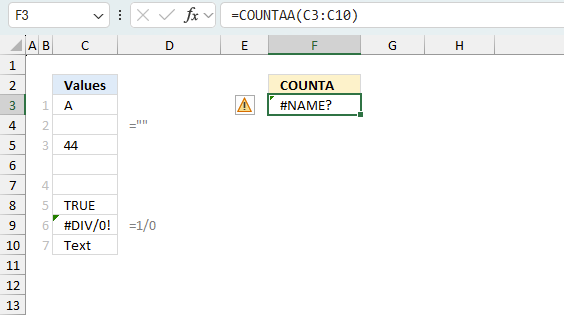
The COUNTA function returns
- #NAME? error if you misspell the function name.
- does not propagate errors, meaning that if the input contains an error (e.g., #VALUE!, #REF!), the function will return the same error.
13.1 Troubleshooting the error value
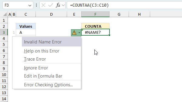
When you encounter an error value in a cell a warning symbol appears, displayed in the image above. Press with mouse on it to see a pop-up menu that lets you get more information about the error.
- The first line describes the error if you press with left mouse button on it.
- The second line opens a pane that explains the error in greater detail.
- The third line takes you to the "Evaluate Formula" tool, a dialog box appears allowing you to examine the formula in greater detail.
- This line lets you ignore the error value meaning the warning icon disappears, however, the error is still in the cell.
- The fifth line lets you edit the formula in the Formula bar.
- The sixth line opens the Excel settings so you can adjust the Error Checking Options.
Here are a few of the most common Excel errors you may encounter.
#NULL error - This error occurs most often if you by mistake use a space character in a formula where it shouldn't be. Excel interprets a space character as an intersection operator. If the ranges don't intersect an #NULL error is returned. The #NULL! error occurs when a formula attempts to calculate the intersection of two ranges that do not actually intersect. This can happen when the wrong range operator is used in the formula, or when the intersection operator (represented by a space character) is used between two ranges that do not overlap. To fix this error double check that the ranges referenced in the formula that use the intersection operator actually have cells in common.
#SPILL error - The #SPILL! error occurs only in version Excel 365 and is caused by a dynamic array being to large, meaning there are cells below and/or to the right that are not empty. This prevents the dynamic array formula expanding into new empty cells.
#DIV/0 error - This error happens if you try to divide a number by 0 (zero) or a value that equates to zero which is not possible mathematically.
#VALUE error - The #VALUE error occurs when a formula has a value that is of the wrong data type. Such as text where a number is expected or when dates are evaluated as text.
#REF error - The #REF error happens when a cell reference is invalid. This can happen if a cell is deleted that is referenced by a formula.
#NAME error - The #NAME error happens if you misspelled a function or a named range.
#NUM error - The #NUM error shows up when you try to use invalid numeric values in formulas, like square root of a negative number.
#N/A error - The #N/A error happens when a value is not available for a formula or found in a given cell range, for example in the VLOOKUP or MATCH functions.
#GETTING_DATA error - The #GETTING_DATA error shows while external sources are loading, this can indicate a delay in fetching the data or that the external source is unavailable right now.
13.2 The formula returns an unexpected value
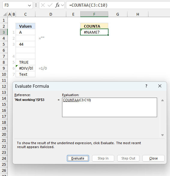
To understand why a formula returns an unexpected value we need to examine the calculations steps in detail. Luckily, Excel has a tool that is really handy in these situations. Here is how to troubleshoot a formula:
- Select the cell containing the formula you want to examine in detail.
- Go to tab “Formulas” on the ribbon.
- Press with left mouse button on "Evaluate Formula" button. A dialog box appears.
The formula appears in a white field inside the dialog box. Underlined expressions are calculations being processed in the next step. The italicized expression is the most recent result. The buttons at the bottom of the dialog box allows you to evaluate the formula in smaller calculations which you control. - Press with left mouse button on the "Evaluate" button located at the bottom of the dialog box to process the underlined expression.
- Repeat pressing the "Evaluate" button until you have seen all calculations step by step. This allows you to examine the formula in greater detail and hopefully find the culprit.
- Press "Close" button to dismiss the dialog box.
There is also another way to debug formulas using the function key F9. F9 is especially useful if you have a feeling that a specific part of the formula is the issue, this makes it faster than the "Evaluate Formula" tool since you don't need to go through all calculations to find the issue..
- Enter Edit mode: Double-press with left mouse button on the cell or press F2 to enter Edit mode for the formula.
- Select part of the formula: Highlight the specific part of the formula you want to evaluate. You can select and evaluate any part of the formula that could work as a standalone formula.
- Press F9: This will calculate and display the result of just that selected portion.
- Evaluate step-by-step: You can select and evaluate different parts of the formula to see intermediate results.
- Check for errors: This allows you to pinpoint which part of a complex formula may be causing an error.
The image above shows cell reference B3:B10 converted to hard-coded value using the F9 key.
Tips!
- View actual values: Selecting a cell reference and pressing F9 will show the actual values in those cells.
- Exit safely: Press Esc to exit Edit mode without changing the formula. Don't press Enter, as that would replace the formula part with the calculated value.
- Full recalculation: Pressing F9 outside of Edit mode will recalculate all formulas in the workbook.
Remember to be careful not to accidentally overwrite parts of your formula when using F9. Always exit with Esc rather than Enter to preserve the original formula. However, if you make a mistake overwriting the formula it is not the end of the world. You can “undo” the action by pressing keyboard shortcut keys CTRL + z or pressing the “Undo” button
13.3 Other errors
Floating-point arithmetic may give inaccurate results in Excel - Article
Floating-point errors are usually very small, often beyond the 15th decimal place, and in most cases don't affect calculations significantly.
Back to top
'COUNTA' function examples
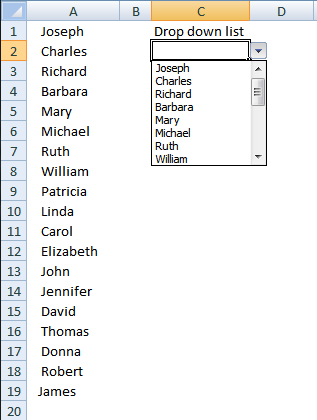
Table of Contents Add values to a regular drop-down list programmatically How to insert a regular drop-down list Add values […]
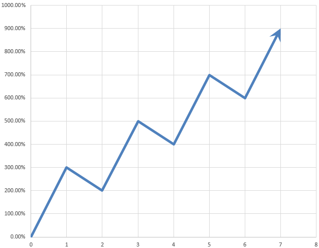
Table of Contents Automate net asset value (NAV) calculation on your stock portfolio Calculate your stock portfolio performance with Net […]
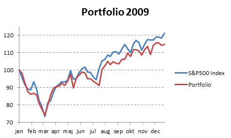
Table of Contents Compare the performance of your stock portfolio to S&P 500 Tracking a stock portfolio in Excel (auto […]
Functions in 'Statistical' category
The COUNTA function function is one of 73 functions in the 'Statistical' category.
How to comment
How to add a formula to your comment
<code>Insert your formula here.</code>
Convert less than and larger than signs
Use html character entities instead of less than and larger than signs.
< becomes < and > becomes >
How to add VBA code to your comment
[vb 1="vbnet" language=","]
Put your VBA code here.
[/vb]
How to add a picture to your comment:
Upload picture to postimage.org or imgur
Paste image link to your comment.
Contact Oscar
You can contact me through this contact form