How to use the CHOOSECOLS function

What is the CHOOSECOLS function?

The CHOOSECOLS function returns given columns from a cell range or array.

The image above shows a set of values in cell range B2:D5, I have enetered a CHOOSECOLS formula in cell B9:

It spills values to cells below and to the right of cell B9 as far as needed, this is done automatically. This specific formula in cell B9 extracts columns 2 and three from B2:D5.

The CHOOSECOLS function is available to Excel 365 users and is in the "Array manipulation" category.

 

1. Syntax

CHOOSECOLS(array, col_num1, [col_num2], …)

Back to top

2. Arguments

array	Required. The source cell range or array.
col_num1	Required. A number represents the column in a given cell range.
[col_num2]	Optional. Extra column numbers to be extracted.

Back to top

3. Example

The picture above shows how the CHOOSECOLS function extracts the second and third column from cell range B2:D5.

Dynamic array formula in cell B9:

The image contains numbers below each column in cell range B2:D5, the numbers lets you easily identify columns 2 and 3. The output is shown in cell B9, columns 2 and 3 are extracted from B2:D5.

Excel 365 dynamic array formulas are different than regular array formulas. The former are entered as regular formulas, however they automatically spill values below and to the right as far as needed. A #SPILL! error is displayed if a cell is not empty where spilling needs to be returned. Simply delete the value and the formula works again.

3.1 Explaining formula

Step 1 - CHOOSECOLS function

The CHOOSECOLS function has two required arguments and one optional. The optional argument is not limited to one value, it can be up to at least 254 arguments.

CHOOSECOLS(array, col_num1, [col_num2], …)

Step 2 - Populate arguments

array - B2:D5
col_num1 - 2
[col_num2] - 3

Step 3 - Evaluate function

CHOOSECOLS(B2:D5, 2, 3)

becomes

CHOOSECOLS({89, 27, 26;
68, 84, 98;
19, 92, 62;
37, 63, 45}, 2, 3)

and returns

{27, 26; 84, 98;
92, 62; 63, 45}

The image below shows the array in cell range B9:C12.

Back to top

4. How to combine specific cell range columns - CHOOSECOLS Function

The CHOOSECOLS function lets you use an array in the arguments, the image above demonstrates a CHOOSECOLS function that uses an array in the second argument. This means that you are not limited to arguments, you can use an array in one argument. This makes it possible to use a lot more than 254 columns.

Dynamic array formula in cell B9:

The image above has values in cell range B2:D5, I have entered blue numbers below each column so you can more easily see the extracted columns. Columns 1 and 3 are returned to a dynamic array that spills values to cells below and to the right as far as needed.

This makes the CHOOSECOLUMNS function useful for combining specific columns from a given data set., this in return makes it even easier to work with arrays in Excel 365 than in earlier Excel versions.

Explaining formula

Step 1 - Populate the array

The curly brackets let you build an array that you can use in most but not all Excel functions. The ; semicolon is a delimiting character that separates values row by row.

The CHOOSE function requires numbers separated with semicolons or whatever row delimiting character you use.

{1; 3}

Step 2 - CHOOSECOLS function

CHOOSECOLS(array, col_num1, [col_num2], …)

CHOOSECOLS(B2:D5, {1; 3})

becomes

CHOOSECOLS({89, 27, 26;
68, 84, 98;
19, 92, 62;
37, 63, 45}, {1; 3})

and returns

{89, 26;
68, 98;
19, 62;
37,45}

Back to top

5. How to combine specific columns based on a given value - CHOOSECOLS Function

The section shows how to return specific columns based on a string containing numbers delimited by a character. The TEXTSPLIT function separates values into an array.

Cell F2 contains the foloowing thext string: 1,2 This string is separated into an array using the comma as a delimiting character. The array is then used to extract columns 1 and 2 from cell range B2:D5.

Dynamic array formula in cell B9:

This is handy if the Excel user needs to specify the given columns in a cell, which in turn makes it more user friendly than editing hard-coded values in a formula. Working with arrays has never been easier, the new Excel 365 functions are very much so appreciated.

Explaining formula

Step 1 - Split text

The TEXTSPLIT function lets you split a string into an array across columns and rows based on delimiting characters.

TEXTSPLIT(Input_Text, col_delimiter, [row_delimiter], [Ignore_Empty])

TEXTSPLIT(F2,,",")

becomes

TEXTSPLIT("1,2", , ",")

and returns {"1"; "2"}.

Note the double quotes, Excel handles these values as text values. The next step converts text values to numbers.

Step 2 - Convert text to numbers

The asterisk lets you multiply numbers in an Excel formula, I am using it here to convert text to numbers.

TEXTSPLIT(F2,,",")*1

becomes

{"1"; "2"}*1

and returns {1; 2}.

Step 3 - CHOOSECOLS function

CHOOSECOLS(B2:D5,TEXTSPLIT(F2,,",")*1)

becomes

CHOOSECOLS(B2:D5, {1; 2})

becomes

CHOOSECOLS({89, 27, 26;
68, 84, 98;
19, 92, 62;
37, 63, 45}, {1; 2})

and returns

{89, 27;
68, 84;
19, 92;
37, 63}

The image below shows the array described above in cell B9, the dynamic array formula spills values cells below and to the right as far as needed.

Back to top

6. How to combine columns using negative values - CHOOSECOLS Function

The CHOOSECOLS function lets you also use negative numbers, this will make the function count columns from right to left.

This is useful if you have a large array containing many columns. If you need to extract columns located to the far right, instead of counting columns from left to right you can use negative integers and count from right to left. This may save you time and less prone to errors.

Formula in cell B9:

CHOOSECOLS(array, col_num1, [col_num2], …)

The image above shows an array in cell range B2:C5. The formula in cell B9 extracts the last column and the next one counting from right to left using negative numbers.

Back to top

7. Function not working

The CHOOSECOLS function returns a #VALUE! error when no values can be displayed.Here is a scenario when this can happen.

The image above displays an array in cell range B2:D5, the formula in cell B9 tries to extract the fifth column from B2:D5, however, there are only three columns in cell range B2:D5.

This makes it impossible for the CHOOSECOLS function to extract the fifth column thus returning the #VALUE error. You can catch errors using the IFERROR function, however, hiding errors is not always great. The downside is that if hide errors you make them much harder to find. Finding errors is most important in order to troubleshoot and find a solution to the problem.

7.1 Troubleshooting the error value

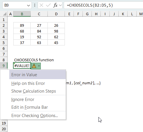
When you encounter an error value in a cell a warning symbol appears, displayed in the image above. Press with mouse on it to see a pop-up menu that lets you get more information about the error.

1. The first line describes the error if you press with left mouse button on it.
2. The second line opens a pane that explains the error in greater detail.
3. The third line takes you to the "Evaluate Formula" tool, a dialog box appears allowing you to examine the formula in greater detail.
4. This line lets you ignore the error value meaning the warning icon disappears, however, the error is still in the cell.
5. The fifth line lets you edit the formula in the Formula bar.
6. The sixth line opens the Excel settings so you can adjust the Error Checking Options.

Here are a few of the most common Excel errors you may encounter.

#NULL error - This error occurs most often if you by mistake use a space character in a formula where it shouldn't be. Excel interprets a space character as an intersection operator. If the ranges don't intersect an #NULL error is returned. The #NULL! error occurs when a formula attempts to calculate the intersection of two ranges that do not actually intersect. This can happen when the wrong range operator is used in the formula, or when the intersection operator (represented by a space character) is used between two ranges that do not overlap. To fix this error double check that the ranges referenced in the formula that use the intersection operator actually have cells in common.

#SPILL error - The #SPILL! error occurs only in version Excel 365 and is caused by a dynamic array being to large, meaning there are cells below and/or to the right that are not empty. This prevents the dynamic array formula expanding into new empty cells.

#DIV/0 error - This error happens if you try to divide a number by 0 (zero) or a value that equates to zero which is not possible mathematically.

#VALUE error - The #VALUE error occurs when a formula has a value that is of the wrong data type. Such as text where a number is expected or when dates are evaluated as text.

#REF error - The #REF error happens when a cell reference is invalid. This can happen if a cell is deleted that is referenced by a formula.

#NAME error - The #NAME error happens if you misspelled a function or a named range.

#NUM error - The #NUM error shows up when you try to use invalid numeric values in formulas, like square root of a negative number.

#N/A error - The #N/A error happens when a value is not available for a formula or found in a given cell range, for example in the VLOOKUP or MATCH functions.

#GETTING_DATA error - The #GETTING_DATA error shows while external sources are loading, this can indicate a delay in fetching the data or that the external source is unavailable right now.

7.2 The formula returns an unexpected value

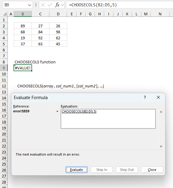
To understand why a formula returns an unexpected value we need to examine the calculations steps in detail. Luckily, Excel has a tool that is really handy in these situations. Here is how to troubleshoot a formula:

1. Select the cell containing the formula you want to examine in detail.
2. Go to tab “Formulas” on the ribbon.
3. Press with left mouse button on "Evaluate Formula" button. A dialog box appears.
   The formula appears in a white field inside the dialog box. Underlined expressions are calculations being processed in the next step. The italicized expression is the most recent result. The buttons at the bottom of the dialog box allows you to evaluate the formula in smaller calculations which you control.
4. Press with left mouse button on the "Evaluate" button located at the bottom of the dialog box to process the underlined expression.
5. Repeat pressing the "Evaluate" button until you have seen all calculations step by step. This allows you to examine the formula in greater detail and hopefully find the culprit.
6. Press "Close" button to dismiss the dialog box.

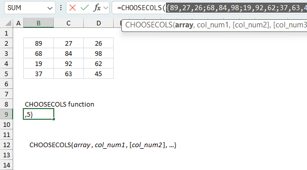
There is also another way to debug formulas using the function key F9. F9 is especially useful if you have a feeling that a specific part of the formula is the issue, this makes it faster than the "Evaluate Formula" tool since you don't need to go through all calculations to find the issue.

1. Enter Edit mode: Double-press with left mouse button on the cell or press F2 to enter Edit mode for the formula.
2. Select part of the formula: Highlight the specific part of the formula you want to evaluate. You can select and evaluate any part of the formula that could work as a standalone formula.
3. Press F9: This will calculate and display the result of just that selected portion.
4. Evaluate step-by-step: You can select and evaluate different parts of the formula to see intermediate results.
5. Check for errors: This allows you to pinpoint which part of a complex formula may be causing an error.

The image above shows cell reference B2:D5 converted to hard-coded value using the F9 key. The CHOOSECOLS function requires a valid col_num1 argument which is not the case in this example. We have found what is wrong with the formula.

Tips!

• View actual values: Selecting a cell reference and pressing F9 will show the actual values in those cells.
• Exit safely: Press Esc to exit Edit mode without changing the formula. Don't press Enter, as that would replace the formula part with the calculated value.
• Full recalculation: Pressing F9 outside of Edit mode will recalculate all formulas in the workbook.

Remember to be careful not to accidentally overwrite parts of your formula when using F9. Always exit with Esc rather than Enter to preserve the original formula. However, if you make a mistake overwriting the formula it is not the end of the world. You can “undo” the action by pressing keyboard shortcut keys CTRL + z or pressing the “Undo” button

7.3 Other errors

Floating-point arithmetic may give inaccurate results in Excel - Article

Floating-point errors are usually very small, often beyond the 15th decimal place, and in most cases don't affect calculations significantly.

Back to top

8. Extract values from given columns and return the list in random order - CHOOSECOLS function

The image above shows an array in cell range B2:D5. The formula in cell B8 returns values in random order from columns two and three in B2:D5.

Dynamic array formula in cell B8:

The result in cell B8 shows an array with the same size as column 2 and 3 from cell range B2;D5. However, the values from column 2 and 3 are in random order. Note that the formula also only returns values from column 2 and 3 but in random order.

8.1 Explaining formula in cell B8

Step 1 - Filter columns 2 and 3

CHOOSECOLS(B2:D5, 2, 3)

becomes

CHOOSECOLS({89, 27, 26;
68, 84, 98;
19, 92, 62;
37, 63, 45}, 2, 3)

and returns

{27,26;
84,98;
92,62;
63,45}

Step 2 - Rearrange values to a single row

The TOROW function rearranges values from a 2D cell range or array to a single row.

TOROW(array, [ignore], [scan_by_col])

TOROW(CHOOSECOLS(B2:D5,2,3))

becomes

TOROW({27,26;
84,98;
92,62;
63,45}

and returns

{27, 26, 84, 98, 92, 62, 63, 45}.

Step 3 - Count cells

The COLUMNS function returns the number of columns in a given cell range or array.

COLUMNS(array)

COLUMNS(TOROW(CHOOSECOLS(B2:D5,2, 3)))

becomes

COLUMNS({27, 26, 84, 98, 92, 62, 63, 45})

and returns 8.

Step 4 - Count rows

The ROWS function returns the number of rows in a given cell range or array.

ROWS (array)

ROWS(CHOOSECOLS(B2:D5,2, 3))

becomes

ROWS({27,26;
84,98;
92,62;
63,45})

and returns 4.

Step 5 - Create random decimal numbers

The RANDARRAY function returns a table of random numbers across rows and columns.

RANDARRAY([rows], [columns], [min], [max], [whole_number])

RANDARRAY(,COLUMNS(TOROW(CHOOSECOLS(B2:D5,2, 3))))

becomes

RANDARRAY(,6)

and returns

{0.215398134613085, 0.390607168196479, ... ,0.83231474462401}.

Step 6 - Rearrange values in random order

The SORTBY function allows you to sort values from a cell range or array based on a corresponding cell range or array.

SORTBY(array, by_array1, [sort_order1], [by_array2, sort_order2],…)

SORTBY(TOROW(CHOOSECOLS(B2:D5,2, 4)),RANDARRAY(,COLUMNS(CHOOSECOLS(B2:D5,2, 3))))

becomes

SORTBY({27,26;
84,98;
92,62;
63,45}, {0.215398134613085, 0.390607168196479, ... ,0.83231474462401})

and returns

{84, 98, 27, 92, 62, 26, 45, 63}

Step 7 - Rearrange values to the original array size

The WRAPCOLS function rearranges values from a single row to a 2D cell range based on a given number of values per column.

WRAPCOLS(vector, wrap_count, [pad_with])

WRAPCOLS(SORTBY(TOROW(CHOOSECOLS(B2:D5,2, 4)),RANDARRAY(,COLUMNS(TOROW(CHOOSECOLS(B2:D5,2, 4))))),ROWS(CHOOSECOLS(B2:D5,2, 3)))

becomes

WRAPCOLS({63, 37, 45, 98, 84, 68}, ROWS(CHOOSECOLS(B2:D5,2, 3)))

becomes

WRAPCOLS({84, 98, 27, 92, 62, 26, 45, 63}, 4)

and returns

{84, 98; 27, 92; 62, 26; 45, 63}.

Step 8 - Shorten formula

The LET function lets you name intermediate calculation results which can shorten formulas considerably and improve performance.

LET(name1, name_value1, calculation_or_name2, [name_value2, calculation_or_name3...])

WRAPCOLS(SORTBY(TOROW(CHOOSECOLS(B2:D5, 2, 3)), RANDARRAY(, COLUMNS(TOROW(CHOOSECOLS(B2:D5, 2, 3))))), TOROW(CHOOSECOLS(B2:D5, 2, 3)))

becomes

LET(z, CHOOSECOLS(B2:D5, 2, 3), x, TOROW(z), WRAPCOLS(SORTBY(x, RANDARRAY(, COLUMNS(x))), ROWS(z)))

Back to top

9. Join multiple non-adjacent cell ranges and return given columns (3D range) - CHOOSECOLS function

The image above shows three data sets in cell ranges B3:D6, F3:H6, and J3:L6. The formula in cell B9 merges these three non-contiguous cell ranges vertically and returns columns 1 and 2.

Dynamic array formula in cell B9:

This is a rather complicated manipultaion of three different cell ranges. The CHOOSECOLS and VSTACK functions makes it super easy to join the cell ranges and then extract only column 1 and 2.

This formula can be really useful if you want to work with cell ranges across multiple worksheets and apply different calculations, for example, like finding the average or return unique distinct values. These types of calculations have never been easier with the new Array manipulation functions.

9.1 Explaining formula

Step 1 - Stack values horizontally

The VSTACK function lets you combine cell ranges or arrays, it joins data to the first blank cell at the bottom of a cell range or array (vertical stacking)

VSTACK(array1, [array2],...)

VSTACK(B3:D6, F3:H6, J3:L6)

becomes

VSTACK({"Peach", 43, 1.03;"Blueberry", 39, 1.48;"Apple", 46, 1.1;"Grapefruit", 14, 0.72}, {"Mandarin", 29, 0.78;"Raspberry", 33, 1.07;"Plum", 25, 0.9;"Mango", 37, 1.13}, {"Pear", 17, 0.63;"Orange", 31, 1.06;"Lime", 17, 1.27;"Kiwi", 45, 0.58})

and returns

{"Peach", 43, 1.03;
"Blueberry", 39, 1.48;
"Apple", 46, 1.1;
"Grapefruit", 14, 0.72;
"Mandarin", 29, 0.78;
"Raspberry", 33, 1.07;
"Plum", 25, 0.9;
"Mango", 37, 1.13;
"Pear", 17, 0.63;
"Orange", 31, 1.06;
"Lime", 17, 1.27;
"Kiwi", 45, 0.58}

Step 2 - Filter given rows

CHOOSECOLS(VSTACK(B3:D6, F3:H6, J3:L6),1, 2)

becomes

CHOOSECOLS({"Peach", 43, 1.03;
"Blueberry", 39, 1.48;
"Apple", 46, 1.1;
"Grapefruit", 14, 0.72;
"Mandarin", 29, 0.78;
"Raspberry", 33, 1.07;
"Plum", 25, 0.9;
"Mango", 37, 1.13;
"Pear", 17, 0.63;
"Orange", 31, 1.06;
"Lime", 17, 1.27;
"Kiwi", 45, 0.58}, 1, 5, 9)

and returns

{"Peach", 43;
"Blueberry", 39;
"Apple", 46;
"Grapefruit", 14;
"Mandarin", 29;
"Raspberry", 33;
"Plum", 25;
"Mango", 37;
"Pear", 17;
"Orange", 31;
"Lime", 17;
"Kiwi", 45}

Back to top

How to use the CHOOSECOLS functionv2

Useful links

CHOOSECOLS function - Microsoft support
CHOOSECOLS Function in Excel: Explained
CHOOSECOLS function in Excel to get columns from array or range

'CHOOSECOLS' function examples

The following article has a formula that contains the CHOOSECOLS function.

Functions in 'Array manipulation' category

The CHOOSECOLS function function is one of 11 functions in the 'Array manipulation' category.

Excel function categories

Excel categories

Leave a Comment