How to use the WRAPROWS function

What is the WRAPROWS function?

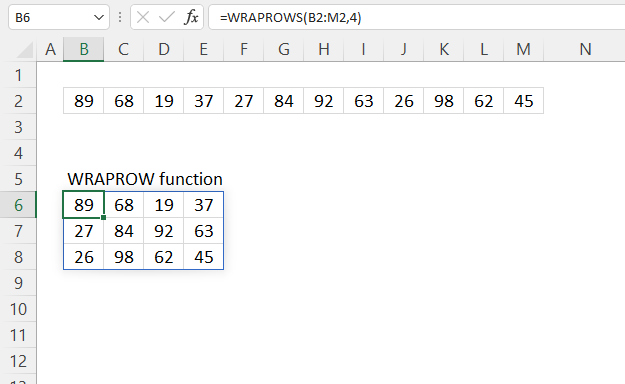
The WRAPROWS function rearranges values from a single row to a 2D cell range.

1. Introduction

Which Excel versions support the WRAPROWS function?

The WRAPROWS function is a new function only available to Excel 365 subscribers.

Which category is the WRAPROWS function in?

The WRAPROWS function is in the "Array manipulation" category.

What is an Excel 365 dynamic formula?

An Excel 365 dynamic array formula is a powerful new feature that allows a single formula to return multiple results across a range of cells automatically. Dynamic array formulas represent a significant change in Excel's functionality allowing for more efficient and flexible spreadsheet design and calculations.

Here are the key aspects of dynamic array formulas:

• Single cell entry: The formula is entered in just one cell, but can output results to multiple cells automatically, this is called spilling.
• Automatic spilling: Results "spill" into adjacent cells automatically without needing to copy the formula in contrast to older Excel versions.
• Dynamic resizing: The output destination range instantly and automatically adjusts as the source data changes.
• No special keystrokes: Unlike traditional array formulas, dynamic arrays don't require Ctrl+Shift+Enter.
• New functions: Excel 365 introduced several new functions designed to work with dynamic arrays, like FILTER, SORT, UNIQUE, etc.
• Works with existing functions: Most existing Excel functions now support dynamic array behavior.
• Easier complex calculations: Dynamic arrays simplify tasks that were previously difficult, like filtering data.
• Backward compatibility: Dynamic arrays are only available in Microsoft 365 versions of Excel, not in older versions like Excel 2019 or 2016.

How do Excel 365 formula handle arrays differently than older Excel versions?

In older Excel versions prior to Excel 365, array formulas worked differently than the dynamic array formulas introduced in Excel 365. Array formulas in older Excel versions required more manual setup and had less flexibility compared to the dynamic array formulas introduced in Excel 365. They were powerful but often more challenging to use and maintain as the user easily could break an array formula by editing the formula in the formula bar.

• Ctrl+Shift+Enter: Array formulas had to be entered by pressing Ctrl+Shift+Enter (CSE) instead of just Enter. This is why they were often called "CSE formulas".
• Pre-selected range: Unlike Excel 365 dynamic arrays users had to pre-select the entire output range before entering the formula.
• No automatic spilling: Results did not automatically spill into neighboring cells. The formula had to be manually copied to fill the desired range.
• Fixed output size: Once entered, the output range was fixed and did not dynamically resize if the source data changed.
• Curly braces: Excel would automatically add curly braces {} around the formula in the formula bar to indicate it was an array formula.
• Complex syntax: Array formulas often required more complex syntax and were more difficult to construct and understand compared to regular formulas.
• Single and multi-cell results: Array formulas could return either a single result or multiple results, depending on how they were constructed and entered.
• Powerful calculations: Despite their complexity, array formulas allowed for powerful calculations and could perform operations on multiple cells simultaneously.
• No specific array functions: Older versions didn't have dedicated array functions like FILTER, SORT, or UNIQUE. Users had to create array formulas using existing functions in creative ways.
• Compatibility: These legacy CSE array formulas are still supported in newer versions of Excel for backward compatibility.

2. Syntax

WRAPROWS(vector, wrap_count, [pad_with])

vector	Required. The source cell range or array.
wrap_count	Required. The number of values per row, the last row may be smaller.
[pad_with]	Optional. Value to pad with if there is an insufficient number of values in the last row. The default value is #N/A!

Back to top

3. Example 1

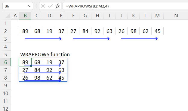
The picture above shows how the WRAPROWS function rearranges values to fit the requirement specified in the second argument: wrap_count.

Dynamic array formula in cell B8:

3.1 Explaining formula

Step 1 - WRAPROWS function

WRAPROWS(vector, wrap_count, [pad_with])

Step 2 - Populate arguments

vector - B2:E4
wrap_count - 4

Step 3 - Evaluate function

WRAPROWS(B2:M2, 4)

becomes

WRAPROWS({89, 68, 19, 37, 27, 84, 92, 63, 26, 98, 62, 45})

and returns

{89, 68, 19, 37; 27, 84, 92, 63; 26, 98, 62, 45}.

Back to top

4. Example 2 - pad with

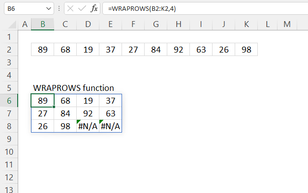
#N/A errors show up in empty cells on the last row, use the [pad_with] argument to populate empty cells.

Formula in cell B6:

The image below demonstrates how to populate empty cells with the text string "A".

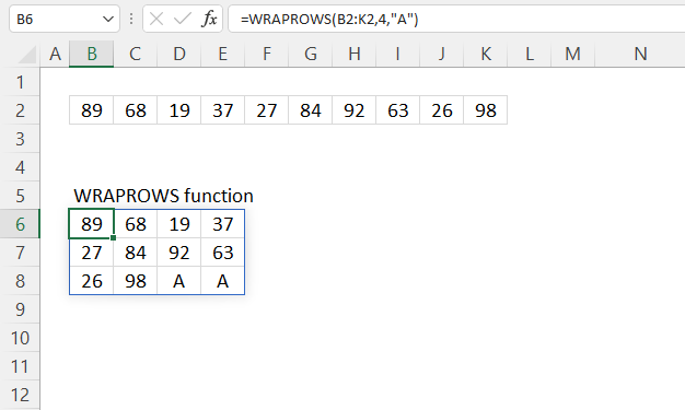
Formula in cell B6:

Back to top

5. WRAPROWS function alternative

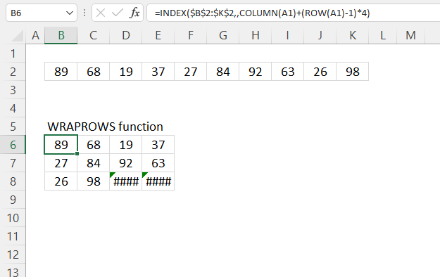
This formula wraps the values in cell range B2:K2 to fit four columns. Change the bolded number in the formula below to adjust the number of columns.

Formula in cell B6:

5.1 Explaining formula in cell B6

Step 1 - Calculate the number of columns in a given cell range

The COLUMN function returns the column number of the top-left cell of a cell reference.

COLUMN(reference)

COLUMN(A1) returns 1.

Step 2 - Calculate column number of relative cell reference

The ROW function returns the row number of a cell reference.

ROW(reference)

ROW(A1)-1

becomes

1 - 1 equals 0 (zero).

Step 3 - Multiply

The asterisk lets you multiply numbers in an Excel formula.

The parentheses controls the order of calculation, we want to subtract before we multiply.

(ROW(A1)-1)*4

becomes

0*4 equals 0 (zero)

Step 4 - Calculate column number

The INDEX function returns a value from a cell range, you specify which value based on a row and column number.

INDEX(array, [row_num], [column_num], [area_num])

INDEX($B$2:$K$2,,COLUMN(A1)+(ROW(A1)-1)*4)

becomes

INDEX($B$2:$K$2,,1)

and returns 89 in cell B6.

Back to top

6. Example 3 - values in random order

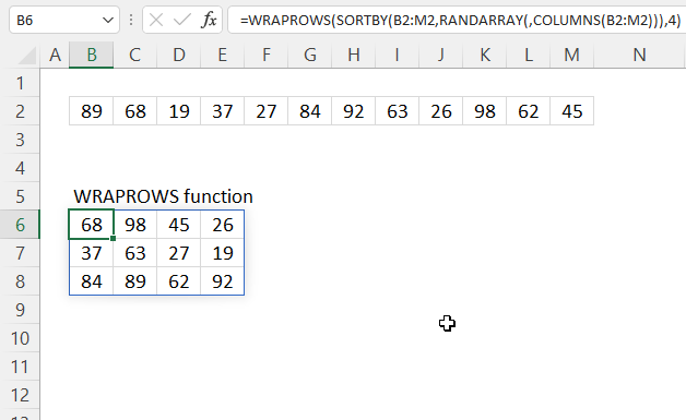
The image above shows a formula that rearranges values in random order with four columns.

Dynamic array formula in cell B6:

6.1 Explaining formula in cell B8

Step 1 - Calculate the number of cells in cell ref

The COLUMNS function returns the number of columns in a given cell range.

COLUMNS(array)

COLUMNS(B2:M2)

returns 12.

Step 2 - Create random decimal values

The RANDARRAY function returns a table of random numbers across rows and columns.

RANDARRAY([rows], [columns], [min], [max], [whole_number])

RANDARRAY(, COLUMNS(B2:M2))

becomes

RANDARRAY(, 12)

and returns

{0.732441255476154, 0.953587479053817, ... , 0.0191675082920368}

Step 3 - Sort values based on random decimals

The SORTBY function allows you to sort values from a cell range or array based on a corresponding cell range or array.

SORTBY(array, by_array1, [sort_order1], [by_array2, sort_order2],…)

SORTBY(B2:M2, RANDARRAY(, COLUMNS(B2:M2)))

becomes

SORTBY(B2:M2, {0.732441255476154, 0.953587479053817, ... , 0.0191675082920368})

and returns

Step 4 - Create random values

The RANDARRAY function returns a table of random numbers across rows and columns.

RANDARRAY([rows], [columns], [min], [max], [whole_number])

RANDARRAY(, ROWS(B2:E4)*COLUMNS(B2:E4))

becomes

RANDARRAY(, 12)

and returns 12 random decimal values:

{0.464680665246457, 0.768212043461448, ... ,0.281771048521311}

Step 6 - Sort values in random order

The SORTBY function allows you to sort values from a cell range or array based on a corresponding cell range or array.

SORTBY(array, by_array1, [sort_order1], [by_array2, sort_order2],…)

SORTBY(B2:M2, RANDARRAY(, COLUMNS(B2:M2)))

becomes

SORTBY(B2:M2, {0.732441255476154, 0.953587479053817, ... , 0.0191675082920368})

becomes

SORTBY({89, 68, 19, 37, 27, 84, 92, 63, 26, 98, 62, 45}, {0.732441255476154, 0.953587479053817, ... , 0.0191675082920368})

{63, 45, 27, 68, 84, 26, 92, 62, 98, 37, 89, 19}

Step 5 - Wrap values

WRAPROWS(SORTBY(B2:M2, RANDARRAY(, COLUMNS(B2:M2))), 4)

becomes

WRAPROWS({63, 45, 27, 68, 84, 26, 92, 62, 98, 37, 89, 19}, 4)

and returns

{63,45,27,68;
84,26,92,62;
98,37,89,19}

Press F9 to recalculate values, this creates a new random order.

7. Example 4 - multiple source ranges

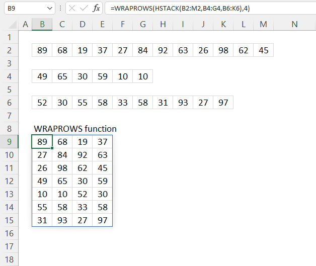
The graphic above demonstrates a formula that merges values from cell ranges B2:M2, B4:G4, and B6:K6, then wraps the values to a 2D range with max four values wide.

Dynamic array formula in cell B6:

7.1 Explaining formula

Step 1 - Stack values horizontally

The HSTACK function lets you combine cell ranges or arrays, it joins data to the first blank cell to the right of a cell range or array (horizontal stacking)

HSTACK(array1, [array2],...)

HSTACK(B2:M2, B4:G4, B6:K6)

becomes

HSTACK({89, 68, 19, 37, 27, 84, 92, 63, 26, 98, 62, 45}, {49, 65, 30, 59, 10, 10}, {52, 30, 55, 58, 33, 58, 31, 93, 27, 97})

and returns

{89, 68, 19, 37, 27, 84, 92, 63, 26, 98, 62, 45, 49, 65, 30, 59, 10, 10, 52, 30, 55, 58, 33, 58, 31, 93, 27, 97}.

Step 2 - Wrap values to rows

WRAPROWS(HSTACK(B2:M2, B4:G4, B6:K6), 4)

becomes

WRAPROWS({89, 68, 19, 37, 27, 84, 92, 63, 26, 98, 62, 45, 49, 65, 30, 59, 10, 10, 52, 30, 55, 58, 33, 58, 31, 93, 27, 97}, 4)

and returns

{89, 68, 19, 37;
27, 84, 92, 63;
26, 98, 62, 45;
49, 65, 30, 59;
10, 10, 52, 30;
55, 58, 33, 58;
31, 93, 27, 97}

Back to top

8. Function not working

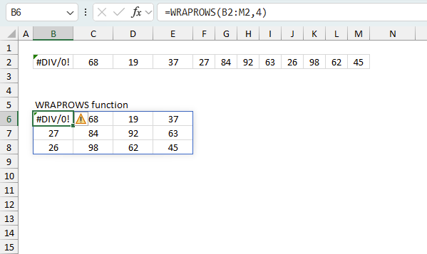
The WRAPROWS function returns

• #NAME? error if you misspell the function name.
• propagates errors, meaning that if the input contains an error (e.g., #VALUE!, #REF!), the function will return the same error.

8.1 Troubleshooting the error value

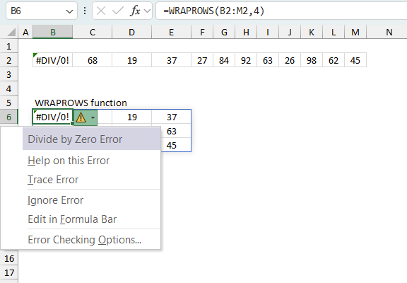
When you encounter an error value in a cell a warning symbol appears, displayed in the image above. Press with mouse on it to see a pop-up menu that lets you get more information about the error.

1. The first line describes the error if you press with left mouse button on it.
2. The second line opens a pane that explains the error in greater detail.
3. The third line takes you to the "Evaluate Formula" tool, a dialog box appears allowing you to examine the formula in greater detail.
4. This line lets you ignore the error value meaning the warning icon disappears, however, the error is still in the cell.
5. The fifth line lets you edit the formula in the Formula bar.
6. The sixth line opens the Excel settings so you can adjust the Error Checking Options.

Here are a few of the most common Excel errors you may encounter.

#NULL error - This error occurs most often if you by mistake use a space character in a formula where it shouldn't be. Excel interprets a space character as an intersection operator. If the ranges don't intersect an #NULL error is returned. The #NULL! error occurs when a formula attempts to calculate the intersection of two ranges that do not actually intersect. This can happen when the wrong range operator is used in the formula, or when the intersection operator (represented by a space character) is used between two ranges that do not overlap. To fix this error double check that the ranges referenced in the formula that use the intersection operator actually have cells in common.

#SPILL error - The #SPILL! error occurs only in version Excel 365 and is caused by a dynamic array being to large, meaning there are cells below and/or to the right that are not empty. This prevents the dynamic array formula expanding into new empty cells.

#DIV/0 error - This error happens if you try to divide a number by 0 (zero) or a value that equates to zero which is not possible mathematically.

#VALUE error - The #VALUE error occurs when a formula has a value that is of the wrong data type. Such as text where a number is expected or when dates are evaluated as text.

#REF error - The #REF error happens when a cell reference is invalid. This can happen if a cell is deleted that is referenced by a formula.

#NAME error - The #NAME error happens if you misspelled a function or a named range.

#NUM error - The #NUM error shows up when you try to use invalid numeric values in formulas, like square root of a negative number.

#N/A error - The #N/A error happens when a value is not available for a formula or found in a given cell range, for example in the VLOOKUP or MATCH functions.

#GETTING_DATA error - The #GETTING_DATA error shows while external sources are loading, this can indicate a delay in fetching the data or that the external source is unavailable right now.

8.2 The formula returns an unexpected value

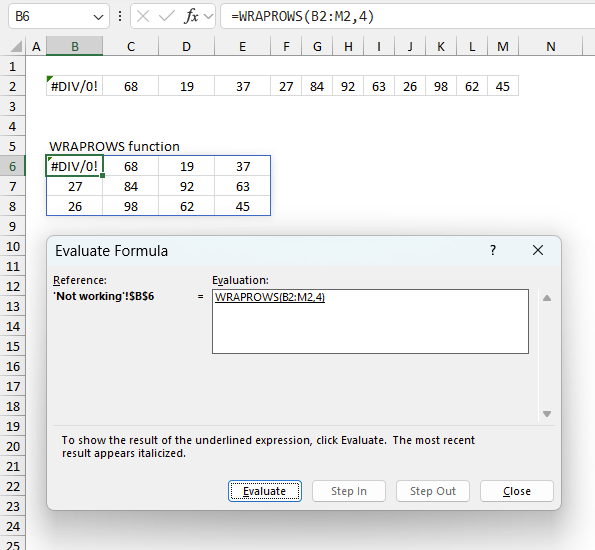
To understand why a formula returns an unexpected value we need to examine the calculations steps in detail. Luckily, Excel has a tool that is really handy in these situations. Here is how to troubleshoot a formula:

1. Select the cell containing the formula you want to examine in detail.
2. Go to tab “Formulas” on the ribbon.
3. Press with left mouse button on "Evaluate Formula" button. A dialog box appears.
   The formula appears in a white field inside the dialog box. Underlined expressions are calculations being processed in the next step. The italicized expression is the most recent result. The buttons at the bottom of the dialog box allows you to evaluate the formula in smaller calculations which you control.
4. Press with left mouse button on the "Evaluate" button located at the bottom of the dialog box to process the underlined expression.
5. Repeat pressing the "Evaluate" button until you have seen all calculations step by step. This allows you to examine the formula in greater detail and hopefully find the culprit.
6. Press "Close" button to dismiss the dialog box.

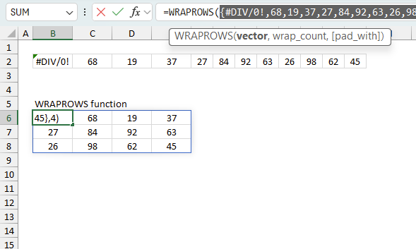
There is also another way to debug formulas using the function key F9. F9 is especially useful if you have a feeling that a specific part of the formula is the issue, this makes it faster than the "Evaluate Formula" tool since you don't need to go through all calculations to find the issue..

1. Enter Edit mode: Double-press with left mouse button on the cell or press F2 to enter Edit mode for the formula.
2. Select part of the formula: Highlight the specific part of the formula you want to evaluate. You can select and evaluate any part of the formula that could work as a standalone formula.
3. Press F9: This will calculate and display the result of just that selected portion.
4. Evaluate step-by-step: You can select and evaluate different parts of the formula to see intermediate results.
5. Check for errors: This allows you to pinpoint which part of a complex formula may be causing an error.

The image above shows cell reference B2:M2 converted to hard-coded value using the F9 key. The WRAPROWS function requires non-error values which is not the case in this example. We have found what is wrong with the formula.

Tips!

• View actual values: Selecting a cell reference and pressing F9 will show the actual values in those cells.
• Exit safely: Press Esc to exit Edit mode without changing the formula. Don't press Enter, as that would replace the formula part with the calculated value.
• Full recalculation: Pressing F9 outside of Edit mode will recalculate all formulas in the workbook.

Remember to be careful not to accidentally overwrite parts of your formula when using F9. Always exit with Esc rather than Enter to preserve the original formula. However, if you make a mistake overwriting the formula it is not the end of the world. You can “undo” the action by pressing keyboard shortcut keys CTRL + z or pressing the “Undo” button

8.3 Other errors

Floating-point arithmetic may give inaccurate results in Excel - Article

Floating-point errors are usually very small, often beyond the 15th decimal place, and in most cases don't affect calculations significantly.

Useful resources

WRAPCOLS function - Microsoft support
Convert column / row to range in Excel: WRAPCOLS & WRAPROWS functions

'WRAPROWS' function examples

The following article has a formula that contains the WRAPROWS function.

Functions in 'Array manipulation' category

The WRAPROWS function function is one of 11 functions in the 'Array manipulation' category.

Excel function categories

Excel categories

Leave a Comment