Match two criteria and return multiple records
This article demonstrates how to extract records/rows based on two conditions applied to two different columns, you can easily extend the formula demonstrated below to include additional criteria.
If you have a scenario where you want to apply multiple conditions on a single column then read this article: Extract all rows from a range that meet criteria in one column [Array formula]
Table of Contents
- Match two criteria and return multiple records [Array Formula]
- Match two criteria and return multiple records [Excel 365]
- Match two criteria and return multiple records [Excel defined Table]
- Match two criteria and return multiple records [Advanced Filter]
- Filter records based on a date range and if a cell value contains a string
- Extract records where all criteria match if not empty
1. Match two criteria and return multiple records [Array Formula]
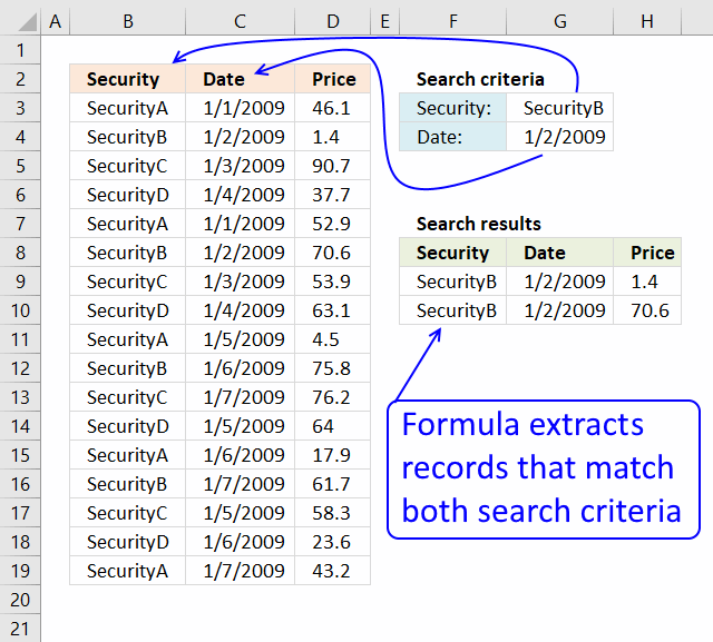
The image above shows you a data set in cell range B2:D19, cell value G3 lets you match values in column B and cell G4 matches dates in column C. The formula returns matching records in cell range F9:H11 when both conditions are met.
1.1 Question
I have a table of 3 columns (Security name, date, price) and I have to find the price of a security at a certain date in a table that contains many securities and prices for these securities for different dates.
If I work with vlookup or Index-match I got only the first price for certain securities. So I am not able to find the price of securities that match both the name of the securities and the date.
Could you advise if there is any way to overcome this?
Array formula in F9:
1.2 Watch a video where I explain the formula
1.3 How to create an array formula
- Copy (Ctrl + c) and paste (Ctrl + v) array formula into formula bar.
- Press and hold Ctrl + Shift.
- Press Enter once.
- Release all keys.
Copy cell F9 and paste it to the right. Copy cell F9:H9 and paste down as far as needed.
1.4 Explaining excel array formula in cell range F9:H10
Use the "Evaluate Formula" tool to examine a formula in great detail. Go to tab "Formulas", press with the mouse on the "Evaluate Formula" button.
A dialog box opens, press the "Evaluate" button to see formula calculations step by step.
Step 1 - First condition
The COUNTIF function calculates the number of cells that is equal to a condition. We can use the COUNTIf function to match the condition to values in cell range B3:B19.
It returns an array containing as many values as there are cells in cell range B3:B19, the values can be 0 (zero) or 1. 1 indicates a match, we can use the array later on to match corresponding row numbers.
The position of a 0 (zero) or 1 in the array is important, the position matches the position in cell range B3:B19.
COUNTIF(range, criteria)
COUNTIF($G$3, $B$3:$B$19)
returns {0; 1; 0; 0; 0; 1; 0; 0; 0; 1; 0; 0; 0; 1; 0; 0; 0}.
Step 2 - Second condition
The second condition is a date specified in cell G4, the COUNTIF function counts the condition against dates in C3:C19.
COUNTIF($G$4, $C$3:$C$19)
returns {0; 1; 0; 0; 0; 1; 0; 0; 0; 0; 0; 0; 0; 0; 0; 0; 0}.
Step 3 - Multiply arrays - AND logic
We need both conditions to be true in order to get the correct values. The asterisk character lets you multiply the array, this is possible because both arrays have the same size.
1 * 1 = 1
1 * 0 = 0
0 * 1 = 0
0 * 0 = 0
COUNTIF($G$3, $B$3:$B$19)*COUNTIF($G$4, $C$3:$C$19)
returns {0; 1; 0; 0; 0; 1; 0; 0; 0; 0; 0; 0; 0; 0; 0; 0; 0}.
Step 4 - Create number sequence
The ROW function calculates the row number of a cell reference. It can also return an array of row numbers if the reference is a cell range.
ROW(reference)
ROW($B$3:$D$19)
returns {3; 4; 5; 6; 7; 8; 9; 10; 11; 12; 13; 14; 15; 16; 17; 18; 19}.
Step 5 - Create number sequence from 1 to n
The MATCH function returns the relative position of an item in an array or cell reference that matches a specified value in a specific order.
MATCH(lookup_value, lookup_array, [match_type])
MATCH(ROW($B$3:$D$19),ROW($B$3:$D$19))
returns {1; 2; 3; 4; 5; 6; 7; 8; 9; 10; 11; 12; 13; 14; 15; 16; 17}.
This array contains row numbers containing as many numbers as there are rows in cell range $B$3:$D$19.
Step 6 - Replace values in array with corresponding row number
Array value 1 is replaced with the corresponding row number. 0 (zero) is replaced with nothing FALSE.
The IF function returns one value if the logical test is TRUE and another value if the logical test is FALSE.
IF(logical_test, [value_if_true], [value_if_false])
IF(COUNTIF($G$3, $B$3:$B$19)*COUNTIF($G$4, $C$3:$C$19), MATCH(ROW($B$3:$D$19),ROW($B$3:$D$19)))
returns {FALSE; 2; FALSE; ... ; FALSE}.
Step 7 - Extract k-th row number
The SMALL function returns the k-th smallest value from a group of numbers. It ignores text and boolean values.
SMALL(array, k)
SMALL(IF(COUNTIF($G$3, $B$3:$B$19)*COUNTIF($G$4, $C$3:$C$19), MATCH(ROW($B$3:$D$19),ROW($B$3:$D$19))), ROWS($A$1:A1))
becomes
SMALL({FALSE; 2; FALSE; ...; FALSE}, ROWS($A$1:A1))
The ROWS function returns the number of rows in a reference, we need the SMALL function to return a new row number in each cell, in order to do that I use the ROWS function and a reference that grows when you copy the formula and paste to cells below.
Reference $A$1:A1 has two parts, an absolute part $A$1 meaning it won't change when the formula is copied to cells below. The second part is a relative reference A1, it changes when the formula is copied.
SMALL({FALSE; 2; FALSE; ....; FALSE}, ROWS($A$1:A1))
returns 2. 2 is the smallest number in the array.
Step 8 - Get value
The INDEX function returns a value from a cell range, you specify which value based on a row and column number.
INDEX(array, [row_num], [column_num], [area_num])
The COLUMNS function works just like the ROWS function except for columns instead, see the explanation above. This allows us to extract the entire row.
INDEX($B$3:$D$19, SMALL(IF(COUNTIF($G$3, $B$3:$B$19)*COUNTIF($G$4, $C$3:$C$19), MATCH(ROW($B$3:$D$19),ROW($B$3:$D$19))), ROWS($A$1:A1)), COLUMNS($A$1:A1))
returns "SecurityB" in cell F9.
1.5 Alternative array formula in F9 [Excel 2007]
Recommended articles
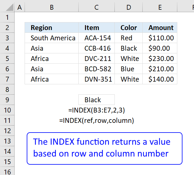
Gets a value in a specific cell range based on a row and column number.
1.6 Excel file
Recommended articles
The following post shows you how to filter records using a single condition:
VLOOKUP - return multiple records
- Extract all rows that contain a value between this and that
- Quickly search a data set with many criteria
- Filter unique distinct records
- Extract duplicate records
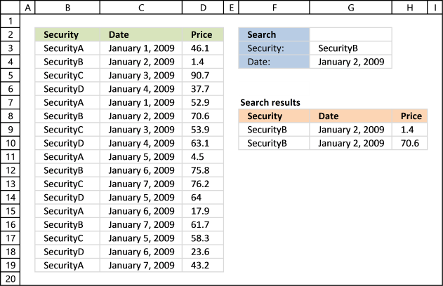
2. Match two criteria and return multiple records [Excel 365]

Dynamic array formula in cell F9:
2.1 Explaining formula in cell F9
Step 1 - First condition
The equal sign is a logical operator that lets you compare value to value. In this case, a value to multiple values, the result is an array containing boolean values True or False.
G3=B3:B19
returns {FALSE; TRUE; FALSE; ... ; FALSE}.
Step 2 - Second condition
The second condition identifies cells in cell range C3:C19 containing the date specified in cell G4.
G4=C3:C19
returns
{FALSE; TRUE; FALSE; ... ; FALSE}.
Step 3 - AND logic
Both conditions must be met, the asterisk character allows you to multiply the arrays meaning AND logic is applied.
TRUE * TRUE = TRUE (1)
TRUE * FALSE = FALSE (0)
FALSE * TRUE = FALSE (0)
FALSE * FALSE = FALSE (0)
When boolean values are multiplied their numerical equivalents are returned. TRUE = 1 and FALSE = 0 (zero).
(G3=B3:B19)*(G4=C3:C19)
returns {0; 1; 0; ... ; 0}.
Step 4 - Extract records
The FILTER function lets you extract values/rows based on a condition or criteria. It is in the Lookup and reference category and is only available to Excel 365 subscribers.
FILTER(array, include, [if_empty])
FILTER(B3:D19, (G3=B3:B19)*(G4=C3:C19))
returns {"SecurityB", 45659, 1.4; "SecurityB", 45659, 70.6}.
2.2 Excel file
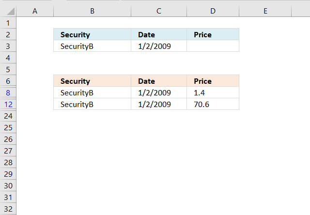
3. Match two criteria and return multiple records [Excel defined Table]
- Select the range

- Press with left mouse button on "Insert" tab
- Press with left mouse button on "Table"

- Press with left mouse button on OK

- Press with left mouse button on black arrow next to header "Security".
- Select the items you want to filter.
- Press with left mouse button on black arrow next to header "Date".
- Make sure only 1-2-2009 is selected.

The image above shows both conditions applied to the Excel Table.
Recommended articles
4. Match two criteria and return multiple records [Advanced Filter]
The image above demonstrates a filter applied to a data set using Excel's Advanced Filter feature. Here is how to create that filter:
- Copy headers and paste to cells below or above the dataset.
Note, the filter values may become hidden if you place them next to the dataset.
- Type the conditions below each header accordingly.
- Select the dataset.
- Go to tab "Data" on the ribbon.
- Press with left mouse button on "Advanced" button, a dialog box appears.
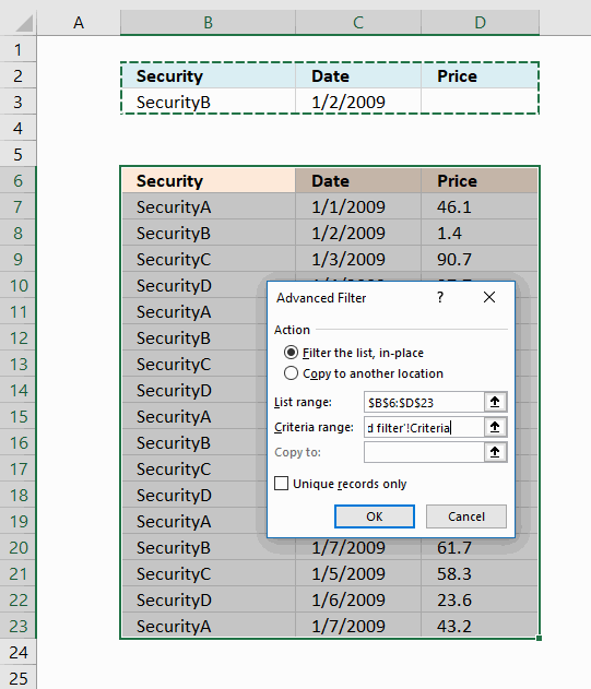
- Press with left mouse button on radio button "Filter the list, in place".
- Press with left mouse button on "Criteria range:" field and select cell range B2:D3, see image above.
- Press with left mouse button on OK button.
The image above shows records filtered on items based on condition in B3 and dates based on condition in C3. If both conditions match on the same row the record/row appears in the filtered list.
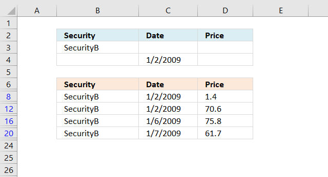
Put the conditions on a row each in order to apply OR-logic instead of AND-logic between conditions, see image below.
Recommended articles
- Extract all rows from a range based on range criteria [Advanced Filter]
- Filter unique distinct values [Advanced Filter]
- Lookup and return multiple values [Advanced Filter]
- Category: Advanced Filter
5. Filter records based on a date range and if a cell value contains a string

Murlidhar asks:
How do I search text in cell and use a date range to filter records?
i.e st.Dt D1 end dt. D2 Search "soft" in entire column for" Microsoft"
Answer:
Excel 365 dynamic array formula in cell F10:
Array formula in cell F10 for earlier Excel versions:
How to create an array formula
- Copy (Ctrl + c) and paste (Ctrl + v) array formula into formula bar.
- Press and hold Ctrl + Shift simultaneously.
- Press Enter once.
- Release all keys.
Copy cell F10 and paste to cell range F10:H12.
Explaining array formula in cell F10
Step 1 - Find cells containing the search string
The SEARCH function returns the number of the character at which a specific character or text string is found reading left to right (not case-sensitive), if string is not found the function returns an error value. If the ISERROR function returns FALSE the logical expression returns TRUE.
ISERROR(SEARCH($G$3, $C$3:$C$29))=FALSE
returns {TRUE; FALSE; TRUE; ... ; FALSE}
Step 2 - Find cells matching dates criteria
The following two logical expressions calculates which records have dates inside the given date range. These two arrays are multiplied to apply AND logic meaning if both logical expressions return TRUE the formula returns TRUE or the equivalent numerical value which is 1. 0 (zero) is FALSE.
($G$4<=$B$3:$B$29)*($G$5>=$B$3:$B$29)
returns {1; 0; 1; ... ; 0}
Step 3 - Convert matching cells and cells containing search string into row numbers
The IF function has three arguments, the first one must be a logical expression. If the expression evaluates to TRUE then one thing happens (argument 2) and if FALSE another thing happens (argument 3). If the ISERROR function returns FALSE (zero) then the IF function returns the corresponding row number.
IF((ISERROR(SEARCH($G$3, $C$3:$C$29))=FALSE)*($G$4<=$B$3:$B$29)*($G$5>=$B$3:$B$29), MATCH(ROW($C$3:$C$29), ROW($C$3:$C$29)), "")
returns {1; ""; 3; ... ; ""}
Step 4 - Return the k-th smallest number
The SMALL function returns the k-th smallest value in the array based on the COLUMN function and a relative cell reference. Then the cell is copied to cells below the relative cell reference changes, this makes the SMALL function return a new value in each cell.
SMALL(IF((ISERROR(SEARCH($G$3, $C$3:$C$29))=FALSE)*($G$4<=$B$3:$B$29)*($G$5>=$B$3:$B$29), MATCH(ROW($C$3:$C$29), ROW($C$3:$C$29)), ""), ROW(A1))
returns 1.
Step 5 - Return a value of the cell at the intersection of a particular row and column
The INDEX function returns a value based on a cell reference and column/row numbers.
INDEX($B$3:$D$29, SMALL(IF((ISERROR(SEARCH($G$3, $C$3:$C$29))=FALSE)*($G$4<=$B$3:$B$29)*($G$5>=$B$3:$B$29), MATCH(ROW($C$3:$C$29), ROW($C$3:$C$29)), ""), ROW(A1)), COLUMN(A1))
returns 40544 (1-Jan-2011).
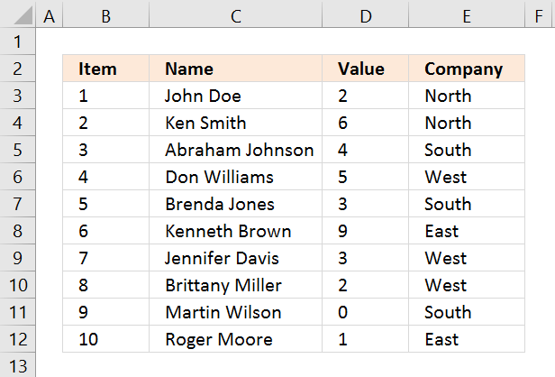
6. Extract records where all criteria match if not empty
![]()
Question: I second G's question: can this be done for more than 3?
i.e.
(Instead of last name, middle, first)
customer#, cust name, appt date, appt time, venue, coordinator, assistant
A question asked in this post:
Lookup with multiple criteria and display multiple search results using excel formula, part 3
Answer:
Array formula in B20:
To enter an array formula, type the formula in a cell then press and hold CTRL + SHIFT simultaneously, now press Enter once. Release all keys.
The formula bar now shows the formula with a beginning and ending curly bracket telling you that you entered the formula successfully. Don't enter the curly brackets yourself.
Excel 365 dynamic array formula in cell B20:
Explaining formula in cell B20
Step 1 - Compare criteria to data
The equal sign allows you to compare values, the resulting array contains TRUE or FALSE.
($B$3:$H$12=$B$16:$H$16)*1
becomes
({1, "Taylor", 39965, ... , 0})*1
becomes
{FALSE, FALSE, FALSE, ...., FALSE}*1
The MMULT function can't work with boolean values so in order to get that working we must multiply the array with 1.
{0, 0, 0, .... , 0}
Step 2 - Add values row-wise
MMULT(($B$3:$H$12=$B$16:$H$16)*1,{1;1;1;1;1;1;1})
returns {0;0;1;0;0;2;1;1;2;1}
Step 3 - Compare sum with the number of criteria
We know a record match if the number of criteria equals the sum returned from the MMULT function. The COUNTA function lets you count non empty cells in a given cell range.
MMULT(($B$3:$H$12=$B$16:$H$16)*1, {1;1;1;1;1;1;1})=COUNTA($B$16:$H$16)
returns {FALSE; FALSE; FALSE; ... ; FALSE}.
Step 4 - Replace TRUE with corresponding row number
The IF function allows you to return a value if the logical expression evaluates to TRUE and another if FALSE.
IF(MMULT(($B$3:$H$12=$B$16:$H$16)*1, {1;1;1;1;1;1;1})=COUNTA($B$16:$H$16), MATCH(ROW($B$3:$B$12), ROW($B$3:$B$12)), "")
returns {"";"";"";"";"";6;"";"";9;""}
Step 5 - Extract the k-th smallest row number
The SMALL function lets you get the k-th smallest number in an array. SMALL( array, k)
SMALL(IF(MMULT(($B$3:$H$12=$B$16:$H$16)*1, {1;1;1;1;1;1;1})=COUNTA($B$16:$H$16), MATCH(ROW($B$3:$B$12), ROW($B$3:$B$12)), ""), ROWS($A$1:A1))
The ROWS function returns the number of rows in a cell reference, this particular cell reference is expanding when the cell is copied to cells below.
SMALL({"";"";"";"";"";6;"";"";9;""}, 1)
and returns 6.
Step 6 - Return value
The INDEX function returns a value from a cell range or array based on a row and column number.
INDEX($B$3:$H$12, SMALL(IF(MMULT(($B$3:$H$12=$B$16:$H$16)*1, {1;1;1;1;1;1;1})=COUNTA($B$16:$H$16), MATCH(ROW($B$3:$B$12), ROW($B$3:$B$12)), ""), ROWS($A$1:A1)), COLUMNS($A$1:A1))
returns "6" in cell B20.
Get Excel *.xlsx file
Filter records category
This article explains different techniques that filter rows/records that contain a given text string in any of the cell values […]
Lookup with criteria and return records.
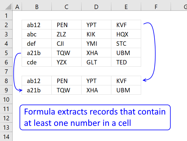
This article describes a formula that returns all rows containing at least one digit 0 (zero) to 9. What's on […]
Excel categories
207 Responses to “Match two criteria and return multiple records”
Leave a Reply
How to comment
How to add a formula to your comment
<code>Insert your formula here.</code>
Convert less than and larger than signs
Use html character entities instead of less than and larger than signs.
< becomes < and > becomes >
How to add VBA code to your comment
[vb 1="vbnet" language=","]
Put your VBA code here.
[/vb]
How to add a picture to your comment:
Upload picture to postimage.org or imgur
Paste image link to your comment.
Hi Oscar, love your blogs! great tutorials. Keep them coming!
Chrisham,thanks!
Thank you for the example. However I stillhave a problem that do not fit on your examples.
I have a table of 3 coloms (Security name, date, price) and I have to find the price a a security at a certain date in a table that contain many securities and prices for this securities for different dates. If I work with vlookup or Index-match I got only the first price for a certain securities. So I am not able to find the price of a securities that match both the name of the securities and the date. Could you advice if there is any way to overcome?
Paolo,
See this blog post: https://www.get-digital-help.com/2010/02/11/match-two-criteria-and-return-multiple-rows-in-excel/
Hi Oscar,
I've got a problem using your suggested approach. I have a list which I need to search from. I have three search criteria, and wish to output a fourth item. For each combination of the search criteria, there will only be one matching result.
I'm trying to use a series of search criteria (arranged in a table - with one row for each search instance, one column for each criterion) which is located on a different worksheet within the same workbook to the data table from which I need to extract the values.
The first search returns the desired result, however the next row returns #NUM error. In order to replicate the formula on the second and subsequent rows I've used a straight forward copy/past - the formula appears to be an Array one still (preceded and suceeded by {} as appropriate).
Do you have any suggestions which might help?
Do you have any suggestions on what might be causing this?
Oscar, your blogs do stretch make my Excel understanding. I have learnt a lot, especially in the usage of these powerful Array formulas. Thanks
In this case its your results would be great for producing a filter list of the criteria mentioned. However if you looking for just a price based on the criteria mentioned, this formula would be more simpler.
=INDEX($D$3:$D$19,MATCH($G$3&$G$4,$B$3:$B$19&$C$3:$C$19,0))
But I guess, the above formula does not work for multiple items of the same criteria....... sorry, I long way to go for me:)
Problem description (simplified of course):
I have a list of employees (by ID number) and date (by yr & mon) of when they were assigned a certain duty (task). This is in a Work book, on a TAB. Each TAB is a separate month (first is Jan, 2nd is Feb, etc.). I have 12 tabs (12 worksheets) in workbook. Each TAB, a single month, has a list of ID numbers. Some IDs may repeat on different worksheets, that is, some may be in multiple months and some may be in just two or three months or just one month. An ID number will shown only once in a month for a single task (duty). Abbreviated example is below.
Is it possible to combine the data, by function, or formula, or VBasic) to a 13th worksheet automatically and:
1. Show a list of all ID numbers in order (without repeating).
2. Show Jan data in col B, Feb data in col C, etc., and some columns will be blank because the ID had no assignment that month, and will not be on the worksheet for that month.
Is there a formula, or function, or does it have to be done in VBasic? (Is it even possible?)
I have the workbook with 12 tabs in it, and now have to manually put the ID columns side by side and copy and slide down one side on the other to get them to match, and repeat the process 12 times to get the yearly data on one worksheet.
Ex:
For Jan:
ID Duty Asgn.
01 C
05 F
09 D
15 X
23 P
For Feb:
ID Duty Asgn.
02 M
05 Q
08 A
12 R
20 W
Combing Jan and Feb would be:
ID Duty Asgn.
01 C
02 M
05 F Q
08 A
09 D
12 R
15 X
20 W
23 P
This would be repeated for each month to build all 12 col months.
Very Respectfully,
Dave Bonar
(504) 697-2395
Dear sir
If you send the excel file, then I'll understand easily and give the better formula. Based on your requirements
Thankyou
Dave Bonar,
Yes, I believe this can be automated using vba. Some of the actions required can also be automated using excel formulas.
Very interesting questions! I´ll try to answer your questions as soon as possible here on my website.
/Oscar
Dave Bonar,
See this post: https://www.get-digital-help.com/2010/02/28/combine-data-from-multiple-sheets-in-excel/
/Oscar
Oscar,
You are doing exacting what I have been trying to do for my Excel file but I cannot seem to get mine to work for some reason. Do you think you could take a look at my file if you have a chance. I would greatly appreciate it.
Bryant,
https://www.get-digital-help.com/contact/
Hello, Oscar,
First of all id like to thank you for your blog. I have found many very usefull tips and answers, but still i have one problem that i cant solve by my self. So im asking for your help.
Here is the problem:
i have a data table with 2 columns:
A B
2.93 12.8
2.94 12.2
3 8.38
3.03 6.76
3.04 5.33
3.06 6.36
Lets say i have a cell with number 3. I need to find a number in column A that has a number >= than 3, but also has the smallest number in column B.
(with my cell = 3 it would be 3.04 from A and 5.33 from B)
Simple vlookup gives me first >= number, but in most cases in column B is not the smalest number.
I hope you can help me,
Best regards,
Liudas
Liudas,
see this post: https://www.get-digital-help.com/2010/03/24/lookup-using-two-criteria-in-excel/
hi oscar,
1) am interested to know what is the array formula for only 1 criteria (for example above, Security, only?
2) how to remove/hide the #num! ?
thanks
David,
1) See this post: https://www.get-digital-help.com/how-to-return-multiple-values-using-vlookup-in-excel/
2) Excel 2007: IFERROR(INDEX(tbl, SMALL(IF(COUNTIF($G$3, $B$3:$B$19)*COUNTIF($G$4, $C$3:$C$19), ROW(tbl)-MIN(ROW(tbl))+1), ROW(A1)), COLUMN(A1));"")
Oscar,
Great Work on this one. This fixed one of my remaining bugs in my spreadsheet. Using the example above, how would you sort the results by 'Price' within the formula?
Thanks
Oscar,
Great Work on this one. This fixed one of my remaining bugs in my spreadsheet. Using the example above, how would you sort the results by 'Price' within the formula?
Thanks
Tom,
Try this array formula in cell F9:
=INDEX(tbl, MATCH(SMALL(IF(COUNTIF($G$3, $B$3:$B$19)*COUNTIF($G$4, $C$3:$C$19), $D$3:$D$19), ROW(A1)), $D$3:$D$19, 0), COLUMN(A1)) + CTRL + SHIFT + ENTER
Copy cell F9 and paste it to H9.
Copy cell range F9:H9 and paste it down as far as needed.
Oscar,
This is close to what I need. In my spreadsheet I do not have the Date to sort by. When I remove the *COUNTIF($G$4,$C$3:$C$19) portion it shows all of the particular Securities. So far so good. Now when I have two securities with the same price on different days it is not soring corectly(notice the date cells in the results). If all of the prices are different it works fine.
IFERROR(INDEX(tbl, MATCH(SMALL(IF(COUNTIF($G$3, $B$3:$B$19), $D$3:$D$19), ROW(A1)), $D$3:$D$19, 0), COLUMN(A1)), "")
Thanks
=INDEX(tbl, MATCH(SMALL(IF(COUNTIF($G$3, $B$3:$B$19), COUNTIF($D$3:$D$19, "<"&$D$3:$D$19)+ROW($B$3:$B$19)/1048576), ROW(A1)), COUNTIF($D$3:$D$19, "<"&$D$3:$D$19)+ROW($B$3:$B$19)/1048576, 0), COLUMN(A1))+ CTRL + SHIFT + ENTER
Copy cell F9 and paste it to H9.
Copy cell range F9:H9 and paste it down as far as needed.
Oscar,
Thanks a bunch. I was able to adapt this to my sheet and got it to work perfectly. Your knowledge is a great asset to others.
While I was able to adapt it, I am not quite sure what it was doing. Can you provide some insight on what this bit is doing:
COUNTIF($D$3:$D$19, "<"&$D$3:$D$19)+ROW($B$3:$B$19)/1048576)
Again thanks for your help.
Tom
Tom,
COUNTIF($D$3:$D$19, "<"&$D$3:$D$19) creates an array containing numbers. The numbers indicate the rank each cell value would have if they were sorted from A to Z. Now if there are two identical cell values the array formula (COUNTIF($D$3:$D$19, "<"&$D$3:$D$19) creates two identical rank numbers. That is why you got the wrong date when you had two identical securities with the same price. To create unique rank numbers I added this to the formula: ROW($B$3:$B$19)/1048576
Awsome! Thanks for the explination.
Oscar,
I am on to the next part of my project now.
Is there a way to combine all of the results into a single cell like with a concatenation with out the formula being extremly large and not containing cells with no values or the seperation characters.
In the above array Formula sample Cell H9 would result in:
$1,40, $70,60
I need to do the whole array and the concatenation in a single cell.
I have a sample spreadsheet of exactly what I trying to accomplish, but I do not know how to get it to you.
Thanks,
Tom
Tom,
As far as I know, concatenate can´t be used in array formulas.
Read about: String Concatenation
Hi Oscar,
Are you able to do this formula but instead of using a specific date, use a greater than date?
Arielle,
=INDEX(tbl, SMALL(IF(COUNTIF($G$3, $B$3:$B$19)*COUNTIF($G$4, "<"&$C$3:$C$19), ROW(tbl)-MIN(ROW(tbl))+1), ROW(A1)), COLUMN(A1)) + CTRL + SHIFT + ENTER copied right as far as needed and then copied down as far as needed.
Hi, Can you do this with a greater than date?
Arielle,
Array formula in cell B25:
=SMALL(IF((COUNTIF(Search_customer, Customer)+COUNTIF(Search_cust_name, Cust_name)+COUNTIF(Search_Appt_time, Appt_time)+COUNTIF(Search_venue, Venue)+COUNTIF(Search_Coordinator, Coordinator)+COUNTIF(Search_Assistant, Assistant))*COUNTIF(Search_Appt_date, "<"&Appt_date), ROW(Customer)-MIN(ROW(Customer))+1), ROWS(B24:$B$24)) + CTRL + SHIFT + ENTER. Copy cell b25 and paste it to the cells below, as far as needed.
Hi,
Can you search within the whole excel workbook instead of just the sheet?
thanks
Also, what if I want to search 2 or more words within a column but they are not together (ex. 1 of the cell stated "hamburger, hotdog, soda", can i search for both hamburger and hotdog if are not side by side?)
thanks for your help
Dear Oscar,
Thank you for this blog. I applied the formula as specified below and it worked well for me.
=INDEX(tbl, SMALL(IF(COUNTIF($G$3, $B$3:$B$19)*COUNTIF($G$4, $C$3:$C$19), ROW(tbl)-MIN(ROW(tbl))+1), ROW(A1)), COLUMN(A1))
How would I weak the formula if I want to still match the 2 criterias of your example (i.e. Security and Date) and in addition sort on the price (e.g. increasing prices)?
Thanks,
Boris
Sheet1
A B C D
8 Country Europe
9 Lights 100
10 Type A 200
11
12 Country USA
13 Fuel 40
14 Diesel 200
15
16 Europe Lights Type A 100
17 USA Fuel Diesel 40
Oscar,is there a way to organize this the information into a database format like row 16 onwards,
It picks up all non blanks between the countries putting each line into a separate column.
Ignore the numbers after type a and diesel in the first half.
Boris,
How would I weak the formula if I want to still match the 2 criterias of your example (i.e. Security and Date) and in addition sort on the price (e.g. increasing prices)?
In your example, I think an array formula would be too complicated. I suggest you use an excel table.
Sean,
Formula in cell A19:
Formula in cell B19:
Get the Excel 2007 file *.xlsx
organize-information.xlsx
Oscar,
Thanks. This is very tricky. The row called Country is the dividing line between each section. I am looking to pick up all the non-blank rows between each section. Move everything from column A besides country over to column B. Ignore the amounts in that is in now in column C. My table was slightly wrong. The amount is in the row below country. So the table looks like this.
Country USA
Lights 100
Type A
CFL
Country Europe
Diesel 50.00
Fuel
USA Lights Type A CFL
Europe Diesel Fuel
Is there any to paste screenshots here?
Sean,
If there is not the same number of rows between sections and country is the dividing line, I think vba is the tool for this task.
Sean,
Read this post: Excel udf: Reorganize data
Dear Mr. Oscar,
Here is my problem.
am having col1, col2, col3 and many data below that.
now i want to create 3 data validation.
Source for the First data validation is all col1.
Source for second data validation is col2 which is match with col1.
Source for third data validation is col3 which is match with col1 and col2.
hope this is clear. please help me
[email protected]
how to retrieve a cell value based on other two cell value by using formula (not using VBA)
b e 1
b f 2
d g 1
d h 4
if i enter "b" and "e" means i should get 1
if i enter "b" and "f" means i should get 2
thanks in advance
[email protected]
I a column with over 400 entries. Most of them are 0s. I would like to list the 5 smallest numbers excluding 0s. What is the best possible formula. Thanks
Muhammad Saleem,
read this post: List five smallest numbers, excluding zeros.
Please can someone help me with this:
I need a function (no macros) that will look at D2, go to column B and display everything in column A thats in column B in ascending order by sorting column C. exampl is below
Name group Invested lookup Answer
First Back $5.00 Back Third
Second Back $6.00 Second
Third Back $7.00 First
Forth Front $10.00
Fifth Side $11.00
Sixth SideA $12.00
A B C D E
Name group Invested lookup Answer
First Back $5.00 Back Third
Second Back $6.00 Second
Third Back $7.00 First
Forth Front $10.00
Fifth Side $11.00
Sixth SideA $12.00
Hi,
In your "Security, Date, Price" scenario I want to match only Security role and return multiple rows. I don't want to match Date. Please help
This is tremendously useful... but what if I need to add additional nested criteria, e.g., if ((A and B) or (c))? The use case I have is that I want to create the list based on the following:
Region: Northeast, Mid-Atlantic, Southeast, etc...
Number: Must be greater than the specified number
Flag 1: if it contains an 'x', add to the list
Flag 2: if it contains an 'x', remove from list
I tried nesting the array calculations as follows:
IF((COUNTIF($I$7,'Customer Stats'!$C$2:$C$206)*COUNTIF($B$3,"<"&'Customer Stats'!$D$2:$D$206)) + COUNTIF($B$4, 'Customer Stats'!$J$2:$J$206))
Where $I$7 contains the Region, $B$3 contains the number above which a record must be to qualify, and $B$4 contains an 'x' if we want to match corresponding records in $J$2:$J$206... but apparently I can't nest these array calculations.
If I add it as another * array, I can get the flagged records to show up in the list, but then any record that shows up must be flagged.
Any ideas?
Thanks,
-Adam
srikanth,
Hi,
In your "Security, Date, Price" scenario I want to match only Security role and return multiple rows. I don't want to match Date. Please help
This formula should do it:
You could also use the formula in this post:
How to return multiple values using vlookup in excel
Awesome, but I have one question?
The above formula matches only security role and returning multiple rows, the output is perfectly fine.
what I want is exclude the "security" column itself in output.
Thanks for your valuable time.
Qadeer
Adam,
Check out the attached file:
Adam.xls
Hi Oscar -
Thanks for the sample... so very close, but I need to restrict the list to only the specified region -- even if flag 1 matches. I will play with it a bit and see what I can do, but if you have a quick solution, do let me know!
Thanks again,
-Adam
Got it, I think... this seems to work, but still testing:
=INDEX($A$5:$C$19, SMALL( IF((COUNTIF($A$2,$A$5:$A$19)*($B$5:$B$19>$B$2))+(COUNTIF($A$2,$A$5:$A$19)*ISNUMBER(SEARCH($C$2,$C$5:$C$19))), MATCH(ROW($A$5:$A$19),ROW($A$5:$A$19)), ""), ROW(A1)), COLUMN(A1))
Adam,
Open attached file:
Adam1.xls
Also close... but that sheet requires the flag to match as well as the region to match... in my code above, I basically * the array, and then add it to a second *'d array, which seems to do the trick. I also subtracted a 3rd *'d array for the list items that we do not want to include no matter what (similar to the flag1 in this example). Only bug seems to be with those list items that have the exclude flag2 set but do not meet the > number requirement, but I can live with that for now... Here is my final code (please excuse the Name references which I added for future maintainability):
=IFERROR(INDEX(AllDataNoHeadings,SMALL(IF((COUNTIF($A$7, AllRegions)*(AllRacks>=$B$3))+(COUNTIF($A$7, AllRegions)*ISNUMBER(SEARCH($N$2,Strategic)))-(COUNTIF($A$7,AllRegions)*ISNUMBER(SEARCH($N$3,NonStrategic))),MATCH(ROW(AllCustomers), ROW(AllCustomers)),""),ROW(A1)),COLUMN(A1)), "")
Thanks again for this excellent website... really helped a lot!
-Adam
This formulas works better then the one I am currently using, it only does one criteria. However I am using the formula on a separate worksheet with my data in a sheet called CSAT Data.
The formula I am using, built from the one in the example, referring to the CSAT Data worksheet will result in a n/a message.
How do we reference the name on a worksheet in the original formula?
Any help would be appreciated!
Ray,
How do we reference the name on a worksheet in the original formula?
Example:
'CSAT Data'!$A$1
Try this syntax (Array formula so remember to C.S.E!)
{=MATCH(B57&C57,B2:B51&C2:C51,0)} for Excel 2007 or higher:
means return the first row number where a value in Col B matches search value in B57 and a a value in Col C matches search value in C57 ON THE SAME ROW!!
Mike,
MATCH(B57&C57,B2:B51&C2:C51,0)} doesn´t work if there are duplicate rows (B2:C51) but with different prices. See row 3 and 7. MATCH(B57&C57,B2:B51&C2:C51,0) returns only the first value.
Thanks for commenting!
Hi!!
This blog is awesome.
How do you return multiple matches in above example, i.e matching 2 criteria by using "SUMPRODUCT" function?
I am trying to match 5 digit numbers to 10 digit numbers in two different excel sheets.
For Example:-
Sheet1:-00085
Sheet2:-9310008522
what function should i use to match these values as data is huge and 5 digit values are also not fixed.
Ramki,
I dont know how.
Why do you want to use sumproduct?
Hi!! Oscar,
Thanks for the reply.
To return multiple values, I felt comfortable with sum product usage.
But I am able to get only Max Value of an array with sum product.
If you help me to get all related multiple values, I would be grateful.
Guarav,
You can use the search function.
Get the example file:
Guarav.xlsx
hello Oscar, i am building a spreadshet for tracking calls for my local fire depatrment. i have column "a" as incident number. the incident number is a one timme yearly number usage. column "c" is apparatus name and there are 1 of 8 possible names may be used in this cell. column "h" has the formula to give me the time spent on scene. i am needing help getting sheet 2 to tag the time spent on a call per apparatus. sheet 2 is names of personnel on scene. i want to put the time on scene according to what apparatus they were on for each incident.
ecample:
column "a" newest entry is #10
column "c" is "bt1" or "bt2" or "e1" or "e3" or "e4" or "e5" or "pov" or "stby"
there often will be multiple rows with the same incident# in column "a" but differant apparatus in column "c".
Column "h" will have on scene time calculated by "=f5-d5"(for that row)
i need to tag the on sceen time from sheet 1 column "h" to the corrisponding incident number column "a" according to the apparatus column "c".
Last Total
Enroute Arrival Clear Response Incident
Incident # Date Apparatus Time Time Time Time Time
1 03/01/12 bt2 8:18 8:27 18:45 0:09:00 10:27:00
2 03/25/12 bt2 8:20 8:23 17:45 0:03:00 9:25:00
e1 17:05 17:10 17:45 0:05:00 0:40:00
e3 12:33 12:38 17:45 0:05:00 5:12:00
3 03/26/12 e4 7:45 8:08 10:22 0:23:00 2:37:00
4 03/26/12 bt2 11:14 11:16 11:29 0:02:00 0:15:00
5 03/27/12 pov 13:10 13:20 18:36 0:10:00 5:26:00
stby 13:15 13:20 18:36 0:05:00 5:21:00
bt1 13:15 13:20 18:36 0:05:00 5:21:00
bt2 13:16 13:21 18:36 0:05:00 5:20:00
6 03/28/12 e1 8:18 8:27 18:45 0:09:00 10:27:00
e3 8:20 8:30 18:45 0:10:00 10:25:00
7 03/28/12 bt1 8:20 8:23 17:45 0:03:00 9:25:00
e5 9:00 9:03 17:45 0:03:00 8:45:00
8 03/28/12 bt2 9:20 9:22 9:59 0:02:00 0:39:00
9 03/29/12 e1 17:45 17:50 18:00 0:05:00 0:15:00
Bill Truax,
read this post:
Tracking calls in excel
Hi Oscar,
Just come across your blog - very useful, and I intend to get stuck into it. I've a quick question on the use of Sum If and And that I can't find on your site. I have the following spreadsheet example
Jan Ann 5
Jan Mike 6
Jan Pete 7
Feb Ann 8
Feb Mike 9
Feb Pete 10
March Ann 11
March Mike 12
March Pete 13
I'm looking for a function where I can search for Feb, and Mike and return the number 9
I feel this is a bit lowbrow for your site - but I'm stuck on it - sorry
Thanks
Ray
For the sake of clarity - they were supposed to show as separate columns - so the month is in column A, Name in Column B, and number in column C
Found the solution within the blog - using SUMIFS - tks for the content
Hi Oscar,
I have been looking at your example today and scratching my head about why it doesn't work in my version of excel. Finally, I've come to the conclusion that this must have something to do with the fact that I looked at your workbook in my German Language Version of Excel.
Somehow the formulas, especially SMALL, don't seem to update their relative reference when I do the Array.
Just for the sake of knowing... you don't perform anything other then a CTRL+ALT+RETURN when creating the Array, right?
Cheers,
Lukas
Hi Oscar,
Sorry for the earlier post. Feel free to delete it. I've just learned that I simply need to create the array in a single cell and then copy it down.
Thanks for the article! Very interesting stuff!
Lukas
Hi Oscar,
How to show the result of the array formula on new worksheet in the same file?
Hi Oscar,
Please ignore my previous post. I wanted to ask about two possibilities about the array formula explained for Security.xlsx file.
1) How to display the result on new worksheet in the same file?
2) I want to search records for the month of January in your example file?
I want to know the solution ASAP.
Look forward to your help in this matter.
Cheers,
M. Nadeem Bhatti.
Hi Oscar,
Any chance this could be modified to generate the resulting list across multiple tabs, 23 rows per tab?
So the formulas in the second tab would ignore the first 23 matching results, and the formulas in the third tab would ignore the first 46 results, etc.
Thanks,
...using the array, that is.
Pivot Tables and macros are not an option for this particular workbook.
thanks
Hi,
I have a model that has three workbooks. Workbook 1 and 2 contains different data sets – there are only two columns in worksheet 1 that can be matched to worksheet 2. Worksheet 3 is my summary page where i am displaying results.
I do require the data be tested for conditions – that is, I am only interested in a row in Worksheet 2 that has two specific columns that match two specific columns in a row in Worksheet 1. I want to view a certain cell of each of these rows where the condition has been proved.
This problems is similar to the one posted at the inception of this thread, however i require greater flexibility in criteria. Essentially i require for each row in worksheet 2 to be scanned against worksheet 1 and, when the above criteria is satisfied, display a cell from that matching row.
Please see below for a portion of the data. Imagine that each of the tables are in different worksheets.
I want certain cells in worksheet 2 from rows where: ‘tenant name’ in worksheet 2 matches ‘building/tenant’ in worksheet 1 and where ‘premises’ in worksheet 2 matches ‘suite id’ in worksheet 1. Curlington Legal Consulting is an example of such a match.
This is required as i need data from one worksheet, however the other contains critical search data.
I also require an additional screening - that is, i do not require any data from worksheet 1 (even if both previous fields have been met) if the expiry is greater than six months away.
Can anyone propose some formulas that could retrieve what i need?
All help is greatly appreciated. It has many people at my firm stumped!
Tony,
I am not sure I am following but I gave it a try:
Tony.xlsx
Beth,
Two or three tabs maximum using array formulas, I think:
Vlookup across multiple sheets in excel
Muhammad Nadeem Bhatti,
1) How to display the result on new worksheet in the same file?
Adjust cell references. Example:
2) I want to search records for the month of January in your example file?
Thanks Oscar,
how do i upload a file to show you specifically what i mean?
Hello Oscar,
I want to search a first vertical range, and then a second vertial range, and then referce the cell in the third column for which the range searches are true.
e.g. I search range A1:A10 looking for the value 1, and find it in A1 and A2. Now I want to narrow this down by searching range B1:B10 (I am actually searching B1:B2 now) to find a second value and find it in B2. So the value I want to refence in C2. How do I achieve this. It is similar to your first example except in my case, AX and BX will always be unique and I want to reference cell CX.
Where do I put "tbl (B3:D19)" to define the range of my table?
Hi Oscar, thanks for your help.
As i cannot upload your file with changes, i will try to describe what i mean.
I guess it's important to say that you were so close - the structure of your worksheets was spot on!
Please note, however, that the matching data will not be in the same rows on each worksheet. In your initial attempt, all matching ‘tenant name’ and premises’ are in the same rows of each data worksheet. Everything else you assumed, however, is perfect.
It is also important to note that where there has been a match found in worksheet 1 and 2 for ‘tenant name’ and ‘premises’, this will be unique. In such an event, I would like other data returned from worksheet one, like what has been done in your first model.
As stated previously, i really want a solution that essentially scans each row individually over every row in worksheet 2, and where a match found, other data from worksheet 1 is displayed in worksheet 3. It would be a good if there was a controlled error message (i.e. how you can display desired text in '=if=' functions) where data is not found, so that i can then sort the results page by a particular metric, unless of course you have a more elegant solution.
Also, as I am a naive excel user, why does this type of syntax require “Ctrl + Alt + Enter” to perform its function. Why won’t it work without it? What is so different in function about an ‘array’ formula?
Thanks again Oscar.
Hi Tony,
I´ll answer your questons as soon as I can. You can use this this contact form to upload your file: Contact form
Tony,
Take a look at this file: Tony_v2.xlsx
Tieku,
Array formula:
The formula returns values from cell range $D$3:$D$19 where $G$3 = $B$3:$B$19 and $G$4 = $C$3:$C$19.
I need to return a value from nine columns based on the following criteria:
Matching an Origin Zip Code (one column)
Matching a Destination Zip Code (one column)
Weight of a shipment (values are split out in nine columns based on weight ranges: 0-500, 501-1000, 1001-2000, etc.
To further complicate this, I need to calculate in a 40% discount on the rate returned (weight column) and add a 17% fuel service charge.
HELP!!!! LOL
Karen G,
Interesting question, can you provide some example data and the desired outcome?
Good morning! I'd be happy to. I work in supply chain logistics and am putting together a decision tool to determine the best way to ship goods. We can ship either Full Truck (FT) or Less Than Truckload (LTL). I have a LTL Tariff Schedule which shows the cost of shipping between two different zip codes, based on various weight ranges. The value is 'pennies per 100 weight', and is the first step in calculating the cost for shipping the product. After the weight 'range' is determined, I have to deduct our average discount (40%) and add back the estimated fuel surcharges (17.5%).
I have the calculation part of this done: =(F13923/100)*(500/100)*0.6*1.175
What I'm struggling with is creating a formula to match the two zip codes, and find the correct 'weight' from the column ranges.
It might be easier if you open Excel and enter this information:
COLUMN HEADERS
A:Origin Zip
Origin St
Dest Zip
Dest St
0-500
501-1000
1001-2000
2001-5000
5001-10000
ROW DATA
1566 MA 500 NY55 4629 3575 2723 2406 1728
COLUMN HEADERS
A: Origin Zip
B: Origin St
C: Dest Zip
D: Dest St
E: 0-500
F: 501-1000
G: 1001-2000
H: 2001-5000
I: 5001-10000
ROW DATA
A: 1566
B: MA
C: 500
D: NY55
E: 4629
F: 3575
G: 2723
H: 2406
I: 1728
The result of this Tariff Schedule needs to be pulled into another document, similar to VLOOKUP. I need to use the Origin Zip (our distribution center), the Destination Zip (customer's distribution center) and weight of shipment to calculate the correct cost of each shipment.
COLUMN A COLUMN B COLUMN C COLUMN D COLUMN E
Customer Customer DC Origin Zip Dest Zip Weight
CVS Bessemer, AL 35023 46158 35023 1005
CVS Conroe, TX 77385 46158 77385 500
COLUMN F = Returns Cost of Shipment from Tariff Schedule outlined in previous post above.
I hope this makes sense!!!!
Hi All - I'd like to search on 2 criteria in a list of data held on a second worksheet and where those 2 criteria are satisfied return the results held in a 3rd cell on the secondary worksheet - there may be multiple true results and the list im looking at is arranged in a vertical list - I want the results pulled through and concatenated into a single cell if possible. I've been all around the answer and had almost the right answer but sadly now my brain has exploded with frustration. Any help may result in the provision of beer or chocolate!!!
Karen G,
See attached file:
KarenG.xlsx
Thank you so much! We're almost there!! The calculation is off by one cell/line. Your formula returned 2723 between zip codes 46158 and 35023; however, the real number should be 1826. Your formula returned the weight for 2000 pounds between the first set of zip codes (01566 and 00500).
Origin Zip Dest Zip Weight Cost of Shipment
46158 35023 1005 2723 (your formula return)
Origin Zip Origin St Dest Zip Dest St 500 1000 2000
1566 MA 500 NY55 4629 3575 2723
46158 35023 AL 2025 1826 7864
How can the numbers in Row 1 Cells E-I act as the decider for the actual weight?
Greetings!! We have figured it out and I wanted to share what we did with you. Hopefully this can help someone else too.
We concatenated both Zip Codes to create one unique primary key: 46158 - 35000
Then created a unique VLOOKUP chart in addition to the LTL Tariff Schedule:
Weight Value Columns
500 2
1000 3
2000 4
5000 5
10000 6
20000 7
30000 8
40000 9
The following VLOOKUP formula was created using the zip code primary key and actual weight of the shipment.
=VLOOKUP(I2,'LTL Tariff Schedule'!$E$2:$M$77025,'LTL Calculation'!J2,FALSE)
WORKS LIKE A CHARM!!!!
Thank you so very much for taking time to try to help me. I greatly appreciate it!
Karen G,
I think I forgot to tell you the formulas in the attached file are array formulas.
I hope this picture explains why the formula returned 7864 for cost of shipment:
Origin Zip Dest Zip Weight Cost of Shipment
46158 35023 1005 2723 (your formula return)
Also, see the weight ranges in row 6.
Dear Oscar,
I m working on the below table.
ORDER MODEL MATERIAL QTY STATUS
BOM a s6 1 COMPLETED
BOM b c6 2 NOT COMPLETED
BOM c s6 1 COMPLETED
DEL d c6 3 NOT COMPLETED
EXP a a8 4 IN PROGRESS
DEL b d2 5 COMPLETED
DEL c c6 4 NOT COMPLETED
DEL d s6 7 NOT COMPLETED
DEL e c6 8 NOT COMPLETED
DEL r a8 1 COMPLETED
EXP g d1 5 COMPLETED
EXP r c6 9 COMPLETED
EXP t a8 2 COMPLETED
EXP a c6 1 NOT COMPLETED
EXP b s6 9 COMPLETED
EXP c c6 1 NOT COMPLETED
EXP d a8 4 NOT COMPLETED
I need the status column to be vlooked up on another file by comparing all the remaining 4 columns.(the sheet to be updated carries the 4 columns not in the same order as in the original sheet.. its mixed).. Pls help me with dis..
Thanks
S.Babu
Try concatenating several fields together to make one (unique) primary key. Example PO number and customer number.
S.Babu,
read this post:
Lookup multiple values in different columns and return a single value
Oscar, great tutorial but i have one question.
In your spreadsheet at the top of the article your search results show a 3rd line that show #NUM1 for each answer.
Is there a way to show this as a blank cell instead?
cheers
Mark,
Yes!
=IFERROR(array_formula, "")
Don´t forget to enter it as an array formula. It works only in excel 2007 and 2010.
sorry #NUM1 should be #NUM!
cheers
I have problem, and o dont know how to solve it, i have data of almost 10000 forms, from which i have to fine 1500, so it is very difficult to dig out 1500 one by one through Ctrl+F, is there any way to to put all the forms number at once and then find all those just by pressing. the prinary key is Form Number
Mohsin Ali Raziq,
I think you will find this post interesting:
Return multiple values using vlookup
Mohsin Ali Raziq,
Read this post:
Quickly search a table using many criteria
Hi Oscar
I have a table on one tab with a list of actions and when they are due to start and when they have been completed with a description. I am creating a cover page on the first tab to show just the last 7 days action descriptions and the next 7 days planned action descriptions for a management summary
I can't seem to work out how I return all the Action descriptions from today and the last 7 days for completed and tomorrow and the next 7 for planned. Can an Array do this?
S.Zeb,
Can an Array do this?
Yes, see attached file:
Filter-dates.xlsx
Thanks Oscar, works a treat. Now have a fully functional automatic dashboard of time specific activities on my spreadsheet header page.
Cheers
[...] Records, Search/Lookup, Sort values on Sep.21, 2012. Email This article to a Friend Mohsin Ali Raziq asks:I have problem, and o dont know how to solve it, i have data of almost 10000 forms, from which i [...]
Hi Oscar,
I'm trying to implement something similar, but using the customer name and between 2 different date ranges, so will need to use >= Appt date1 and <= Appt date2. I've been trying and trying but keep getting the good old #NUM! error!!!
Please help!
Thank you!!!
John
John,
See attached file:
Lookup-with-multiple-criteria-and-display-multiple-search-results-using-excel-formula-part-4-john.xlsx
Hi Oscar,
I really appreciate you getting back to me. Thanks for the file but testing the formula is not producing the results I expect. Let's just simplify the formula and use only the following 3 criteria:
=IFERROR(SMALL(IF(ISNUMBER(SEARCH(Search_cust_name,Cust_name)*COUNTIFS(Appt_date,">="&Search_Appt_date1)*COUNTIFS(Appt_date,"= Search_Appt_date1 AND <= Search_Appt_date2. The string in Search_cust_name MUST match exact. The way the formula is right now still generates results if part of the Search_cust_name parameter matches and even worst if all the criteria values are blanks.
I hope I am explaining myself correctly. Your assistance will be forever appreciated!!!
Thank you,
John
Sorry, that didn't post correctly. I'm going to try again...
Please ignore previous post as it got truncated. Hopefully this will post properly:
Hi Oscar,
I really appreciate you getting back to me. Thanks for the file but testing the formula is not producing the results I expect. Let's just simplify the formula and use only the following 3 criteria:
=IFERROR(SMALL(IF(ISNUMBER(SEARCH(Search_cust_name,Cust_name)*COUNTIFS(Appt_date,">="&Search_Appt_date1)*COUNTIFS(Appt_date,"= Search_Appt_date1 AND <= Search_Appt_date2. The string in Search_cust_name MUST match exact. The way the formula is right now still generates results if part of the Search_cust_name parameter matches and even worst if all the criteria values are blanks.
I hope I am explaining myself correctly. Your assistance will be forever appreciated!!!
Thank you,
John
Hi Oscar,
Just wanted to let you know that my issue has been resolved so please disregard. I was able to incorporate your idea and nested a few other formulas to control the accuracy of the matching results that I expect. Once again thank you for your time as it is very much appreciated!
John
John,
I am going to answer your question anyway. The following formula filters records that exactly match (case insensitive) a criterion or criteria. An empty criteria is not calculated.
Array formula in cell B25:
See attached file:
Lookup-with-multiple-criteria-and-display-multiple-search-results-using-excel-formula-part-4-john.xls
Sorry Oscar but I must be providing a special tag in my post that is messing it all up and it doesn't make sense.
To clarify, let's just simplify the formula so it only checks for an exact match of the Search_cust_name AND between Search_Appt_date1 AND Search_Appt_date2. The way the formula is right now still generates results if part of the Search_cust_name parameter matches and even worst if all the criteria values are blanks.
Please advise and my apologies for the confusion with all the messed up posts!
John
Hi Oscar,
Thank you very much for that solution. it solved my problem !
Just one more question, and I am not sure if the above solution will work here. The problem is with regards to analysing the remaining life of my inventory based on the quantity available and the monthly consumption. Its as follows :
Assuming today's date is 1st of September. I have 20 packets of cheese and the average monthly consumption is 4 packets. Ideally if the shelf life of those 20 packets is 6 months or more, then I can safely say that the total quantity will last for 5 months (20 divided by 4).However, with a slight twist in the data, assume that out of those 20 packets, 6 packets expire on 15 Oct, 7 packets expire on 10 Nov, and the remaining 6 on 15 December. Now I know that the total inventory is not gonna last for 5 months due to various expiry dates. If I calculate this manually, I come to know that the quantity will last for 3 and a half months.
How can i put all this in a formula to get the right answer ?
Please advise.
Thanks
Haroun
Haroun,
See this post:
Inventory consumption
[...] in Count values, Dates, Excel on Oct.05, 2012. Email This article to a Friend Haroun asks:The problem is with regards to analysing the remaining life of my inventory based on the quantity [...]
[...] Search Formula Hi, I wonder whether someone may be able to help me please. From this site Lookup with multiple criteria and display multiple search results using excel formula, part 4 | Get ... I've put together this formula, which works as expected: [...]
Hi Oscar,
I'm designing a fairly simple sheet to calculate a 'border' around a product . There are 3 different materials that can be used, each with a different price per metre. On the sheet, I have a box for user input as to which frame they'd like to use.
I'm now stuck trying to work out which function will allow the sheet to recognise which size material has been used (I used a drop-down box so the user can make a choice from 3 options) and then calculate the total cost from the option they choose. I have all the values in place (options 1,2,3 and cost per ,metre) but I don't which function to use in the calculation box.
This is probably a really simple operation but I've never had to calculate something like this.
Thanks for any help you can offer
Andrew,
Drop down list in cell C2.
Formula in cell C4:
=INDEX(B10:B12,MATCH(C2,A10:A12,0))
Awesome post, thank you so much this is exactly what I needed!
[...] Match two criteria and return multiple rows in excel [...]
Hello Oscar,
I know very little about excel...and seeking your expert advice regarding the below scenerio....
I got 2 spread sheets.
1st one with 50000 rows and columns upto CJ
2nd one with 3000 rows and same number of columns
I need to extract rows from the 1st spreadsheet using values from column CI from the 2nd spreadsheet.
values are not numericals. How can I do it?
ahmed,
Are you comparing values in column CI in both sheets?
Perhaps you can use the method described in this post:
Quickly compare two tables in excel 2007
Use countif instead of countifs.
Dear Oscar,
Can you help me to Retrieve a row details based on three conditions, out of that two will have in the same column and the third one on another, thanks in advance. Regards;
Dear Oscar,
I myself modified your formula to suit my requirements of 3 conditions, however kindly advise my if sorting can be done based on Ascending.
Example:
=INDEX(tbl,SMALL(IF(OR(COUNTIF($C$12,$C$40:$C$84),COUNTIF($C$13,$C$40:$C$84))*COUNTIF($D$19,$D$40:$D$84),ROW(tbl)-MIN(ROW(tbl))+1),ROW(A1)),COLUMN(A1))
Regards
Sudhakar
Hello Oscar,
First off, Thanks for all the great help you do on your website. This website has helped me countless times.
Here is my questions. It's similar to this post.
I wrote a vba macro that searches a column in a data range for a specific number. When it finds any row matching that number it copies that row and pastes it onto another tab, making a list. My goal is to allow people to make changes to that row of data (on the new tab) then when finished, update those specific rows on to the original data range via a "submit button". The problem i'm facing is that when they decide they want to update these rows, i need update the rows that match two specific columns. I'm aware of how to do the replacing of the row when I find the rows that match, but i'm unaware of how to find those rows and have it return to me the row number i need to replace.
Example of main data range
Project Project# Employee Hours
BestBuy 54511 Miguel 20
BestBuy 54511 Martha 10
BestBuy 54511 John 40
WalMart 14513 John 30
WalMart 14513 Martha 10
WalMart 14513 Miguel 70
Example of results when they search for a specific Project#
Project Project# Employee Hours
BestBuy 54511 Miguel 20
BestBuy 54511 Martha 10
BestBuy 54511 John 40
Example of changes they wish to submit back into master (AT THIS POINT IS WHERE I NEED TO FIND THE ROW NUMBER OF ROWS THAT MATCH PROJECT# & EMPLOYEE)
Project Project# Employee Hours
BestBuy 54511 Miguel 70
BestBuy 54511 Martha 0
BestBuy 54511 John 30
Example of UPDATED main data range
Project Project# Employee Hours
BestBuy 54511 Miguel 70
BestBuy 54511 Martha 0
BestBuy 54511 John 30
WalMart 14513 John 30
WalMart 14513 Martha 10
WalMart 14513 Miguel 70
Hope you can help me out, Let me know if you have any other questions or need me to clarify something.
Hi Oscar,
the definition is: COUNTIF(range,criteria)
but from your formula it looks like you are using:
COUNTIF(criteria,range)
ie above: COUNTIF($G$3, $B$3:$B$19)
What you are doing on your awesome blog posts does work so I was just wondering if you could shed more light on it?
Thanks!
Patrick
hello Oscar sir,
i want your argent help
i want to create 1 formula
ex.
if i get value in one cell 2 then it will ans 3
i get 4 or 5 it will return 6
if i get value 7 or 8 then it will return 9
so it will possible then plz reply fast
Siddharth,
Array formula in cell B2:
thank you so much, it solves my problem beautifully
gilgamesh,
Thank you!
Hi Oscar,
Thanks very much for this informative guide. I found it very helpful, and although I just need a bit of help with a certain problem.
I used your array formula with great success to find the search results from multiple critera. However my problem is modifying your formula. In the above example you have shown us, you have two criteria. And you distinguish the two criteria by using *.
My question is: what would you do if you don't know the predetermined number of criteria. So lets say the person searching only specifies security and not date. Or only date, and not security. Or maybe both. The problem is you don't know from before hand.
How would you go about solving this probem?
Your help is greatly appreciated, thanks so much!!
Rashid,
Great question! This post explains to some degree what you are asking for:
Lookup using multiple conditions
Thanks for the quick response Oscar,you have greatly helped me many times over.
I will take a look at the link provided, thanks very much!
Rashid,
read this post:
Lookup with an unknown number of criteria
https://www.get-digital-help.com/2013/10/18/lookup-with-an-unknown-number-of-criteria/
I was wondering if you can recreate this in Numbers on iPad. I am trying to create a cross platform version, but it says the formulas are not compatible. Can somebody help me with this? Not just this article, but everything dealing with popup menus as well.
Jon E,
I have no clue.
[…] lookup with multiple criteria. Indeed, I think the tutorial in the following link is useful: Match two criteria and return multiple rows in excel | Get Digital Help - Microsoft Excel resource (Using the sample from the above link) BUT sometimes in my case, the Cell G3 and G4 may contain a […]
Dear Oscar,
Let me start by saying thank you for your help.
I have a challenge in which I have been trying to fix for long, but never managed to make it work. Hope you can help.
Excel: 2011 MAC
Info:
Three columns A, B and C of Table "TBL"
Search Criteria: $D$11
Goal:
To load rows from column B into data validation list based on Column A matching $D$11
Can this be done?
Regards
Monzer George Yazigi,
Yes, it can be done. But you need a helper column.
Extract-values-and-use-them-in-a-drop-down-list-data-validation.xlsx
Thanks for your kind help.
Highly appreciated.
Hi Oscar,
I have an issue with a payroll schedule.
The payroll schedule has a number of columns: Employee Code, Pay Code, Hours and Rate. Each employee code could have from 1 to 5 different Pay codes. I want to lookup the employee code, if found then look for pay code number 1, if found; return the code, hours and rate, if not found; return blank. Next row, (same employee); look for paycode number 2 etc to paycode 5. Then next employee etc.
Thank you.
Adam,
I believe this post is helpful:
Return multiple records
Hi Oscar,
Hi,
I have a football data spreadsheet that lists all games since 2000/01 (14 seasons). Every line (game) shows date, home team, home team goals, away team goals, away team & result - H, D or A. Columns are A, B, C, D, E, & F.
What I would like to do is for each occurrence of home team & away team to add the result to the Head2Head field (Column G). So if the two teams have played each other for the last 2 seasons and the home team won both, the Head2Head cell would show HH. Similarly if they have played for 6 seasons it could display something like HHDADH. If they have played more than 6 seasons it should drop the earliest to show the latest 6. The earliest result would be on the left of the cell and the most recent on the right. In the last example if a new game produced a draw HHDADH would become HDADHD.
I am not an excel expert so I'm finding it quite difficult to adapt some of your suggestions on the blog.
Hope I have explained it clearly enough.
Thanks in advance..
Is there a way to create a multiple search field in excel through VBA, which would allow me to enter 3 or 4 different searches at one time and have that data populate in order to compare them. The 3 or 4 different searches are coming from a list of 50 different things, which is why i would like to create a search to narrow it down. Thanks!
[…] table when referencing. This should work for you! --------------------------------- Check out Match two criteria and return multiple rows in excel | Get Digital Help - Microsoft Excel resource for more information on how this array formula […]
Hi Oscar,
I am trying to use similar formulas to these to produce a to do list. I deal with FOI requests, and they get reminders sent out at 10, 15, 17 and 19 days, and are due for response on the 20 day (or earlier).
I want to produce a list on the first tab, looking up info from the log (2nd tab), where a request is due it's equivalent reminder and hasn't already had it, or is due for response that day and hasn't yet been closed.
Tab 2 "RequestLog" - Column B is the reference number - this is what i want in the to-do list
Columns V - Y have a P (tick in wingdings2) if their reminder has been sent
Column AA - Has the closed status of the request (is blank if no response has been sent)
Column AX - Has the days remaining until deadline
On tab 1 i have a column for each of the reminders, i.e. for 10 days I want the reference to show up when AX is 5, V (the 10 day column) is blank and AA is blank. This would be the same for all reminders, just changing the "between" part to relate to the days (i.e. 15 days: 3, 17 days: 1, 19 days: =1)
For the 10 day reminder list, I have used the following formula, which will give me the first instance, but when i copy it down, it just says the same again & again:
=INDEX(RequestLog!$A$8:$AX$1008,MATCH(1,(RequestLog!$AA$8:$AA$1008="")*(RequestLog!$V$8:$V$1008="")*(RequestLog!$AX$8:$AX$1008=5),0),2)
I think i am just missing one tiny piece that will allow it to give what i need. Can you help (and is this enough info)?
Preferably, i would want this to hide errors (N/A's), but i can live with having them there...
Thanks in advance for anything light you can shed...
Sorry, have just re-read my post and realised i pasted completely the wrong formula. this is what i have so far managed to get to show the first instance of a FOI requiring a 10 days reminder:
=INDEX(RequestLog!$A$8:$AX$1008,MATCH(1,(RequestLog!$AA$8:$AA$1008="")*(RequestLog!$V$8:$V$1008="")*(RequestLog!$AX$8:$AX$10085),0),2)
For the other reminder columns, all i would need to change is the numbers after .
I hope this all makes sense.....
Still the wrong one! 3rd time lucky...
=INDEX(RequestLog!$A$8:$AX$1008,MATCH(1,(RequestLog!$AA$8:$AA$1008="")*(RequestLog!$V$8:$V$1008="")*(RequestLog!$AX$8:$AX$10085),0),2)
Ok, this website does something to my formula once i press "add comment! Apologies for the multiple comments/posts.
Basically, for the column AX there should be two brackets, one less than 11 (looking at the above the website doesn't post that symbol) and the other greater than 5.
My question is more about the quantity of criteria, I have a table with a number of types, product, ref numbers etc. and I want to create a separate sheet that has a look up function so I can find a single item that matches 3 different criteria (there are 100's of items some with very minor differences). I know I can do this with MATCH and INDEX but I want to know if there is a way to find the same solution by only entering 2 or the criteria (i.e. all three criteria are available to fill but I only need to enter two for the solution to return.
Thanks in advance.
Hello. I found your article great, as it was just what I needed to figure out. Unfortunately I couldn't get it to work! :( Am I being dim, but the CountIf(criteria, range) just counts the number of instances of of that criteria within the range, does it not, so when I use your splitting up example of (COUNTIF($G$3, $B$3:$B$19)
becomes
COUNTIF("SecurityB", {SecurityA, SecurityB, SecurityC, SecurityD, SecurityA, SecurityB, SecurityC, SecurityD, SecurityA, SecurityB, SecurityC, SecurityD, SecurityA, SecurityB, SecurityC, SecurityD, SecurityA})
and reurns this array: {0, 1, 0, 0, 0, 1, 0, 0, 0, 1, 0, 0, 0, 1, 0, 0, 0}
...just returns '4' for me.
I am not used to working in arrays yet, but I hope to learn! Thank you in anticipation.
This is fantastic. I would like the table to be longer, say through B3:D100. I changed the tbl to include this and the formulas in the countifs to include 100, but it is not coming up with the right information in the search results. Can you help?
Thanks.
PLS HELP ME TO SOLVE THE BELOW:
I NEED TO SEARCH TWO WORKBOOKS, IF A OF 1ST WORKBOOK MATCHES WITH B OF 2ND WORKBOOK THEN IF THE QTY OF C IN 2ND WORKBOOK IS GREATER THAN 1, RETRIVE A RESULT AS 1 OR ELSE 0
Hi Oscar,
Your blog is fantastic. It makes so many things about excel much clearer. I have used this array formula successfully to get information based on 2 criteria and return the outupt in columns, except it does not work past the first row:
{=INDEX(Table24, SMALL(IF(COUNTIFS($A3, customerID, J$1, companyList), ROW(Table24)-MIN(ROW(Table24))), ROW(I2)), 23)}
I removed the +1 you had inside the small because it was returning the next row down for some reason but even when I add it back in the formula does not work past the first row.
I read through all the comments for this thread and your thread on VLOOKUP returning multiple values which seemed to address this problem but none of the suggested tweaks seem to work for me.
Please help.
Good evening Oscar!
Your invaluable tips have been helpful for many enthusiastic excel users like me.
Could you please shed light on a scenario: I want to create an excel sheet "B" which feeds itself from data in sheet "A"(which we don't have to play with). The crux is sheet "A" gets periodically updated and has fixed number of rows; and sheet "B" needs to be auto-updated in its consecutive rows, with it looking up value in sheet 'A" and pasting only new data from sheet 'A". This means number of rows of sheet "B" will be constantly increasing. Can we use some formula that can update sheet "B" with new value from sheet "A" every time we drag down formula in sheet "B"?
Thanks a lot,
Prabin
Prabin
with it looking up value in sheet 'A" and pasting only new data from sheet 'A". This means number of rows of sheet "B" will be constantly increasing.
If I understand you correctly, you can't save old data to a sheet, using a formula. You need a macro to do that.
Thank you for your kind attention Oscar. Any suggestion on what type of Macro could achieve that?
Regards,
Prabin
Hi Oscar,
Great Blog!
I discovered that the formula does not work if you are looking for the same value in different columns.
What I mean is, if I have a table and the same values in two different columns and I would like to return all rows that have the needed value in one of the column the formula will not return anything.
If I change it to be a different value everything works.
Do you happen to know how this could be fixed?
Thanks!
Kobi S.
Here is the original formula:
=INDEX(tbl, SMALL(IF(COUNTIF($G$3, $B$3:$B$19)*COUNTIF($G$4, $C$3:$C$19), ROW(tbl)-MIN(ROW(tbl))+1), ROW(A1)), COLUMN(A1))
If you want to look for the same value in two different columns, use this formula:
=INDEX(tbl, SMALL(IF(COUNTIF($G$3, $B$3:$B$19)*COUNTIF($G$3, $C$3:$C$19), ROW(tbl)-MIN(ROW(tbl))+1), ROW(A1)), COLUMN(A1))
It looks for value in cell G3 in both cell range B3:B19 and C3:C19, if both cells match on the same row the entire record is extracted.
Hi Oscar,
I need to implement a logical OR meaning:
(0,0) = Do not report
(0,1), (1,0) & (1,1) = Report line
I tried changing the "*" between the countif to "+" or using countifs but it did not work.
Any thoughts?
Kobi S.
You are right, use a + sign like this:
=INDEX(tbl, SMALL(IF(COUNTIF($G$3, $B$3:$B$19)+COUNTIF($G$3, $C$3:$C$19), ROW(tbl)-MIN(ROW(tbl))+1), ROW(A1)), COLUMN(A1))
Remember it is an array formula.
Worked like a charm!
Thank you!
Hi
Thank you very much!
It's working.
the same security data , what will be the formula if i want , the records which belong to security B and price greater than $ 40.0
Hi, could you please help me, i need to find a formula that extract and list the different numbers that match with 2 conditions.
To find the work number that match with the date and the area. Thank you,
Graciela
If security is your area condition and date is your date condition and your work numbers are in column D (price in example at the very top of this article)
Array formula:
=INDEX($D$3:$D$19, SMALL(IF(COUNTIF($G$3, $B$3:$B$19)*COUNTIF($G$4, $C$3:$C$19), ROW($B$3:$D$19)-MIN(ROW($B$3:$D$19))+1), ROW(A1)))
Hi Oscar,
great page but I still need help.
I have two tables and I have to find all Connectors/Cross sections combinations in Table 1 and write the terminal number in Table 2 column E
Table 2 Column C "First match"
{=INDEX($A$3:$A$7;MATCH(1;(FIND(","&A12&",";$B$3:$B$7)>0)*(FIND(","&B12&",";$C$3:$C$7)>0);0))}
Table 2 Column D Count
{=SUMPRODUCT(ISNUMBER((FIND(","&A12&",";$B$3:$B$7))*(FIND(","&B12&",";$C$3:$C$7)))*TRUE)}
My problem is to join all found results/terminals together in one cell.
Do you have any suggestion for me?
A B C D E
1 Table 1
2 Terminal Connectors Cross sections
3 Nr1 ,S1,S2,S3, ,0.25,0.75,1.0,
4 Nr2 ,S4,S5,S3, ,0.25,1.0,
5 Nr3 ,S6,S7, ,0.35,0.5,
6 Nr4 ,S4,S8,S9,S10, ,0.5,1.0,
7 Nr5 ,S1,S3, ,0.25,0.75,
8
9
10 Table 2
11 Connector Cross section first match count Expected
12 S1 0.75 Nr1 2 Nr1,Nr5
13 S2 0.5 #N/A 0
14 S3 0.25 Nr1 3 Nr1,Nr2,Nr5
15 S4 1.0 Nr2 2 Nr2,Nr4
16 S5 0.25 Nr2 1 Nr2
17 S6 0.75 #N/A 0
18 S7 0.5 Nr3 1 Nr3
19 S8 0.5 Nr4 1 Nr4
20 S9 0.5 Nr4 1 Nr4
21 S10 1.0 Nr4 1 Nr4
22 S1 0.25 Nr1 2 Nr1,Nr5
Thanks in advance
Stefan
Stefan,
the TEXTJOIN function allows you to concatenate values based on a condition:
https://www.get-digital-help.com/2010/12/20/excel-udf-lookup-and-return-multiple-values-concatenated-into-one-cell/
https://www.get-digital-help.com/2016/06/07/textjoin-function/
Hello Oscar,
thanks for the links.
My problem now is that I do not get the result matrix before joining.
{IF({1;0;0;0;1};$A$3:$A$7;"")}
should return
{Nr1;"";"";"";Nr5}
But it returns only "Nr1"
What I´m doing wrong?
Thanks again for you help.
Hi Oscar,
I´ve got it know. :-)
Thanks for your help.
Stefan
The answer to this is entering the formula as an array formula, if anyone else has this question.
To enter an array formula, type the formula in a cell then press and hold CTRL + SHIFT simultaneously, now press Enter once. Release all keys.
The formula bar now shows the formula with a beginning and ending curly bracket telling you that you entered the formula successfully. Don't enter the curly brackets yourself.
=IFERROR(INDEX(Case, SMALL(IF(MMULT((Case=$B$4:$K$4)*1, {1;1;1;1;1;1;1;1;1;1})=COUNTA($B$4:$K$4), MATCH(ROW(Case), ROW(Case)), ""),ROWS($B$2:B2)), COLUMNS($B$2:B2)), "")
here is my code.
I would like to ask why even though it refers to case(Table), when I add new data to table it can't be found in the search.
even when it's inside the table?
Chiang
The following workbook contains an Excel defined Table:
https://www.get-digital-help.com/wp-content/uploads/2009/10/Lookup-with-multiple-criteria-and-display-multiple-search-results-using-excel-formula-part-4-johnv2_table.xlsx
I would like to ask why even though it refers to case(Table), when I add new data to table it can't be found in the search.
The search seems to work when I add new records to the table, see above workbook.
Hi Oscar,
Thanks for writing this guide. Can I know for the security file what if I want to change the criteria to return results for Security B with prices less than $65? How can I change the formula in cell H9? I've tried changing countif part of it to "<65" but it doesn't seem to work. Thank you!
Winnie Low.
try this:
=INDEX(tbl,SMALL(IF(COUNTIF($G$3,$B$3:$B$19)*COUNTIF($G$4,$C$3:$C$19)*($D$3:$D$19<65),ROW(tbl)-MIN(ROW(tbl))+1),ROW(A1)),COLUMN(A1))
Hi Oscar,
Thank you for the detailed explanation, however, I'm still struggling with applying this formula to the following situation:
Tab 1
Col A Col B Col C
20 A Jake
20 A Jake
20 A Jim
20 A Jake
20 A Mike
20 B Jake
30 A Mike
30 C John
30 C Mike
Tab 2:
Col A Cell B1: A / B / C
20
20
20
20
30
30
30
In tab 2, I need to return the name from column C when col A & B Match the values of col A & cell B1. However, if I return the first name, I want the second return value to be the NEXT DIFFERENT name. Do you have any idea how to assist? It would be amazing if you could help, since I've been struggling with this for a while.
Thank you in advance. Kind regards, Max
Hi Max,
I believe you are looking for this article:
https://www.get-digital-help.com/2010/09/19/vlookup-with-multiple-matches-returns-a-different-value-in-excel/
Hi Oscar,
I have a basic question as I am not able to wrap my head around COUNTIF($G$3, $B$3:$B$19)
Does the range not come up first followed by the criteria? I made a mini table to understand but do not get why we switch the range and the criteria. Please let me know
Adi
Hi Adi,
Yes, the range first and then the criteria.
=COUNTIF (range, criteria)
The COUNTIF function returns an array if you use multiple criteria provided you enter it as an array formula. The array contains the same number of values as there are criteria.
Check out this article for examples:
https://www.get-digital-help.com/2013/03/27/countif-function/
Hello Oscar,
I have adapted your formula to a case of my own but for some reason is not counting the first entry in each of my scenarios in which I am using it. Say I should have 8 results. It skips the first and only shows me the next 7.
Hanna,
Make sure the cell reference in the ROW function points to cell A1 on the first result. The formula will change when you copy the first row of cells and paste them to rows below.
=INDEX($B$3:$D$19, SMALL(IF(COUNTIF($G$3, $B$3:$B$19)*COUNTIF($G$4, $C$3:$C$19), ROW($B$3:$D$19)-MIN(ROW($B$3:$D$19))+1), ROW(A1)), COLUMN(A1))
A better formula is:
=INDEX($B$3:$D$19, SMALL(IF(COUNTIF($G$3, $B$3:$B$19)*COUNTIF($G$4, $C$3:$C$19), ROW($B$3:$D$19)-MIN(ROW($B$3:$D$19))+1), ROWS($A$1:A1)), COLUMNS($A$1:A1))
This formula won't break if you insert rows or columns on the same worksheet.
Hi Oscar
what about below. Is there any similar post I can try out?
Criteria:
First these columns has to be exact matched -(($C$2:$C$12=O2)*($D$2:$D$12=P2)*($E$2:$E$12=Q2)*($F$2:$F$12=R2)*($G$2:$G$12=S2),$B$2:$B$12),1))
Second criteria Column N & B2:B12 : The exact match value the date in column N must not overlap after in B2:B12 in the matched value. See the example above that I have manual enter the map ID
Index match value at A column (Running ID number 0001,0002,0003...) return the A value to column M if above match is matched.
Hi,
Thank you for your video, it has been extremely helpful. I've gotten to the SMALL function piece and I have 3 criteria I'm trying to match on. I have 5 rows that should have data and return the row numbers in the IF statement portion. Am I doing something incorrectly? When I put it in Excel I am using Ctrl+Shift+Enter
=SMALL(IF(COUNTIF(Summary!$C$1,'Cancel Reasons'!$B$3:$B$1173)*COUNTIF(Summary!$C$2,'Cancel Reasons'!$D$3:$D$1173)*COUNTIF(Summary!$C$3,'Cancel Reasons'!$C$3:$C1173),MATCH(ROW($B$3:$B$1173),ROW($B$3:$B$1173)),""),ROWS($A$1:A1))
Hi I have a similar issue. for example i have in column e currencies like usd yen pound
Is it possible to get currency results alphabetically sorted in addition with your results above ?
My goal is to have like a statement of account by currencies
Thank you
Is it possible to make it so that it will search for partial text matches too?
Thank you
Nigel,
Yes, it is possible.
The following array formula in cell B20 returns records that have at least a partial match:
=INDEX($B$3:$H$12, SMALL(IF(MMULT(ISNUMBER(SEARCH($B$16:$H$16, $B$3:$H$12))*($B$16:$H$16<>""), {1;1;1;1;1;1;1})=COUNTA($B$16:$H$16), MATCH(ROW($B$3:$B$12), ROW($B$3:$B$12)), ""), ROWS($A$1:A1)), COLUMNS($A$1:A1))
Limited understanding and I've been struggling with returning a list based on multiple criteria but , thanks to this page, I think I'm making progress.
I'm trying to generate a list based on whether a specified date (in cell H8)between the start dates and end dates for rows on a separate sheet (Date Input). The formula below works but it's based on matching the start dates and matching the end dates. How would I change this to = end dates . I think I'm getting confused 'cos a countif would usually be range first then criteria?
=IFERROR(INDEX('Data Input'!$A$39:$H$536,SMALL(IF(COUNTIF(Sheet1!H$8,'Data Input'!$G$39:$G$536)*COUNTIF(Sheet1!H$8,'Data Input'!$H$39:$H$536),ROW('Data Input'!$A$39:$H$536)-MIN(ROW('Data Input'!$A$39:$H$536))+1),ROW('Data Input'!A6:D6)),COLUMN('Data Input'!A6:D6)),"")
Is it to late to ask questions?
In the
the
>= Appt date1
<= Appt date2
do nothing.
could that be changed to be 2 searches?
thanks
Sorry some how lost the information I was entering.
I have a question using
Lookup-with-multiple-criteria-and-display-multiple-search-results-using-excel-formula-part-4-john.xlsx
in the list where search informaion is entered. 2 of them do not work.
Customer# works ok
Cust name works ok
>= Appt date1 does not work
<= Appt date2 does not work
time works ok
Venue works ok
Coordinator works ok
Assistant works ok
what can I do to fix them?
they are not listed in the results
Row Customer#- Cust name- Appt date- Appt time- Venue - Coordinator- Assistant
Could they be changed to 2 more columns to search and add the results to the results list?
thanks, dean thatcher
HI
Note Appt date works ok in
Lookup-with-multiple-criteria-and-display-multiple-search-results-using-excel-formula-part-4-johnv2_table
hi
How can 3 more search Columns and 3 more results Columns be added to?
Lookup-with-multiple-criteria-and-display-multiple-search-results-using-excel-formula-part-4-johnv2.xlsx
added searches needed would be:
Line
Description
Daily Totals
thanks
hi
How can 3 more search Columns and 3 more results Columns be added to?
Lookup-with-multiple-criteria-and-display-multiple-search-results-using-excel-formula-part-4-johnv2.xlsx
added searches needed would be:
Line
Description
Daily Totals
thanks
hi
How can 3 more search Columns and 3 more results Columns be added to?
Lookup-with-multiple-criteria-and-display-multiple-search-results-using-excel-formula-part-4-johnv2.xlsx
added searches needed would be:
Line
Description
Daily Totals
Hey Oscar.
Fantastic tip thank you! I've managed to integrate with a greater than option, which is working, but I wondered if it was possible to re sort the results rows based on the numerical value of one field.
e.g. search
critera 1
results
result 1 = 8
result 2 = 12
result 3 = 5
result 4 = 22
result 5 = 2
I would like it to be
result 5 = 2
result 3 = 5
result 1 = 8
result 2 = 12
result 4 = 22
Hi Oscar! I really admire your work and all the effort you've put on this website. I have used your worksheet to create a comparison between products of two companies. But i am stuck at one point.
I need to find the closest match of a number (right now it is searching exact match only) on a certain parameter let's say instead of date i have some numbers. How do i do it?
Kindly help me accomplish this task!
Dear sir,
Please help me i need a formula...if my data is in a Colum which is in different cell ..and same data value is down side of coloumn in diffrent row..which is also in diffrent cell...
i need sum of value which three cell data in a cell......
for example....
COLOUM DATA 1 2 3 16 18 20
SUM VALUE 50 500 120 240 240 240
COLOUM DATA SUM VALUE
1-2-3 670
2-3-16 860
3-18-20 600
=COUNTIFS(Roster!J5:J440,'Shift Wise Strength'!A26,Roster!K5:K440,'Shift Wise Strength'!B26,Attendance!S5:S440,"P")
Can someone help me with this ?
why am i not able to get a count on sheet3 of a value from sheet 2 while matching criteria's from sheet 1 & 2 both.
Hello, Oscar! How are you? I hope you're healthy. I thank you for your site and I am enjoying your system applied in the link https://www.get-digital-help.com/lookup-with-multiple-criteria-and-display-multiple-search-results-using-excel-formula-part-4/, however, I have a question about how to fix a problem that it has generated. For example, in the data entry area, if one of the cells is empty (no data, in cell G5, for example) then the cells shows an error "#Num!" in all cells of that row in the search results area or the line information is hidden. Would you know how to help me? Thanks!
I want to search for a specific date, how should i change to get that?
Can someone help me?
I am trying to add an additional matching criteria to my formula.
=IFERROR(INDEX('Sheet 1'!C:C,MATCH(ROWS($2:2),'Sheet 1'!$I:$I,0)),"")
I need somehow add a match is also on CELL A1 in sheet 2
Sheet 1 has a larg list of companies and corresponding data for each company, on sheet 2, I only want to select a specific company from sheet 1 and show the fields from the rows I choose.