Merge tables based on a condition
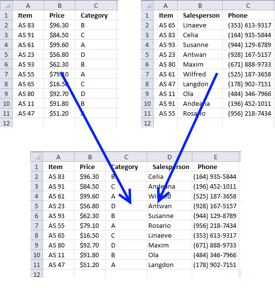
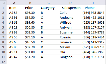
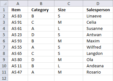
This article demonstrates techniques on how to merge or combine two data sets using a condition. The top left data set has three headers, Item, Price, and Category. The top right data set has three columns, header names are Item, Salesperson, and Phone.
Both data sets contain column Item, this allows you to combine them using the column item as a condition. I will in this article use different Excel functions to merge these data sets. The two last examples show how to combine data sets if a cell contains a given value and how to match multiple columns in order to combine the data sets.
I have written a post about merging two single columns or ranges before: Merge two columns with possible blank cells. It demonstrates how to merge two different columns dynamically and that is it. The following examples merge data tables with a condition or criteria.
What's on this page
- Introduction
- How to join data sets using the VLOOKUP function
- Merge data using the INDEX and MATCH functions
- Merge data sets based on a partial match - wildcard character
- How to merge data using two or more criteria with the COUNTIFS function
- Update list with new values if possible
- Get Excel *.xlsm file
1. Introduction
When can I merge/join combine data from different data sets?
You can merge or combine data when there's a common element between the datasets. This element or "key" can be anything like:
- IDs like Employee ID or Product Code etc
- Dates
- Names
- Categories
Why merge/join combine data from different data sets?
Combining datasets allows you to get a complete picture by connecting related information to make better decisions.
What is a condition in this context?
The condition is the common element between the data sets or the "key".
What is a partial match?
A partial match means you're trying to match part of a string not the whole string.
What is a wild card character?
Wildcards let you match unknown or variable parts of text. Really useful for partial matching.
- * (asterisk) - matches any number of characters, also 0 (zero) characters.
- ? (question mark) - matches one character only
- ~ (tilde) - escapes wild card characters meaning you can search for an asterisk without using it as a wild card character.
2. How to join data sets using the VLOOKUP function
The image above shows two tables on two different worksheets. They only share the same items, however, they are not in order making it harder and tedious to combine manually.
Let us use the Item value in the first table and search for it in the second table. The VLOOKUP function allows us to retrieve corresponding values.
Here is the table in worksheet named sheet1 merged with the table located on worksheet named sheet2, see image above.
Formula in cell D2:
Copy cell D2 and paste to E2. Then copy cell range D2:E2 and paste to cell range D3:E11.
2.1 Explaining formula in cell D2

I do recommend using the "Evaluate Formula" tool when debugging and examining formulas, it allows you to evaluate different parts of the formula individually. Going through the formula is as easy as press with left mouse button oning a button, Excel shows the result of each expression.
Here is how to start this tool. Select the cell you want to check out. Go to tab "Formulas" on the ribbon, press with left mouse button on the "Evaluate Formula" button. This opens a dialog box, see image above.
The "Evaluate Formula" dialog box shows the formula and the underlined expression is what is next to be evaluated, the most recent result from an evaluation is italicized.
Press with left mouse button on the "Evaluate" button to move to the next step in the formula calculation, keep press with left mouse button oning until you are satisfied or the final result appears. That result always match what the cell shows. Press with left mouse button on "Close" button to dismiss the dialog box.
Step 1 - VLOOKUP function

The VLOOKUP function looks for a value in the leftmost column of a table and then returns a value in the same row from a column you specify.
The VLOOKUP function has four arguments: lookup_value, table_array, col_index_num ,range_lookup
VLOOKUP(lookup_value, table_array, col_index_num ,range_lookup)
The Item column is the leftmost column which is needed in order to use the VLOOKUP function, remember the Item column is shared by both data sets.
Step 2 - lookup_value argument
The formula is entered in cell D2 and it uses the corresponding lookup value in cell $A2 to find a match in the second data set located on worksheet Sheet2.
VLOOKUP($A2, 'Ex 1 - Sheet2'!$A$2:$C$11, COLUMN(B1), FALSE)
becomes
VLOOKUP("AS 83", 'Ex 1 - Sheet2'!$A$2:$C$11, COLUMN(B1), FALSE)
See the $ sign? It makes column A absolute, meaning the column part of cell reference does not change when we copy cell D2 and paste to cell E2.
Step 3 - table_array argument
The VLOOKUP function looks for the value in cell $A2 in the leftmost column of cell range 'Ex 1 - Sheet2'!$A$2:$C$11.
It also returns a value from this cell range if there is a match based on the chosen column number in argument col_index_num. See the next step where I explain the col_index_num argument.
VLOOKUP("AS 82", 'Ex 1 - Sheet2'!$A$2:$C$11, COLUMN(B1), FALSE)
Step 4 - col_index_num argument
col_index_num is a column number determining which column in cell 'Ex 1 - Sheet2'!$A$2:$C$11 we want to get values from.
I use COLUMN(B1) in this example, it returns 2 for formulas in column D and 3 for formulas in column E. Cell reference B1 is a relative cell reference meaning it changes when you copy the cell and pastes it to another cell.
Step 5 - range_lookup argument
The range_lookup argument lets you chose if you want the VLOOKUP function to perform an aproximate or exact match. We want an exact match so we will use FALSE.
TRUE - Approximate match
FALSE - Exact match
An approximate match requires the values in the leftmost column in the table_array to be sorted in ascending order. This is not required when you use an exact match.
Step 6 - Return value

The VLOOKUP function finds a match on row 3 and returns the value from the second column on worksheet Sheet2 which is "Celia" and returns that value to cell D2 on worksheet Sheet1.
3. Merge data using the INDEX and MATCH functions
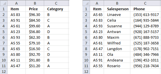
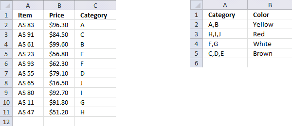
The image above shows two lists on two different sheets. They share the same items, however, they are not sorted. The second list has "Items" in column B (blue circle).
You can't use the VLOOKUP function now unless you move the Items column to the leftmost column in the cell range. But wait, you don't have to move the Items column, you can use a formula that combines two Excel functions.
If you combine the INDEX and MATCH function you can build a formula that is more versatile and as easy to use as the VLOOKUP function. This picture shows the merged list using a formula containing the INDEX and MATCH functions.
Formula in cell D2:
Copy cell D2 to cell range D3:D11.
Formula in cell E2:
Copy cell E2 to cell range E3:E11.
The only difference between these two formulas is the column number that the INDEX function uses to determine which value to extract.
3.1 Explaining formula in cell D2

The following link takes you to an explanation of how the "Evaluate Formula" tool works.
Step 1 - Find the relative position with the value in cell A2 in cell range 'Ex 2 - Sheet2'!$B$2:$B$11
The MATCH function returns a number representing the relative position of a given value (lookup_value argument) in a one-dimensional array or cell range (lookup_array argument).
MATCH(lookup_value, lookup_array, [match_type])
The match_type argument can be -1, 0, and 1. 0 (zero) is an exact match. Check out the other match_type arguments.
MATCH('Ex 2 - Sheet1'!A2,'Ex 2 - Sheet2'!$B$2:$B$11,0)
returns 2. This means that the lookup_value is found in the second position in cell range 'Ex 2 - Sheet2'!$B$2:$B$11 which you can verify if you check out the array above.
Step 2 - Return a value of the cell at the intersection of a particular row and column
The INDEX function returns a value from a cell range or array based on a row and column number (both optional).
INDEX(array, [row_num], [column_num])
INDEX('Ex 2 - Sheet2'!$A$2:$C$11,MATCH('Ex 2 - Sheet1'!A2,'Ex 2 - Sheet2'!$B$2:$B$11,0),1)
returns value "Celia" from row 2 and column 1 in cell range 'Ex 2 - Sheet2'!$A$2:$C$11.
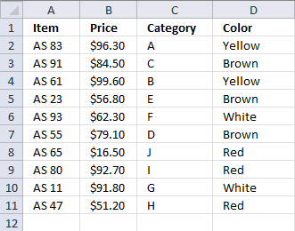
4. Merge data sets based on a partial match - wildcard character
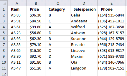
Here we want to find the color for each category, the first data set contains category values in the third column. The second list contains multiple categories in column A and a corresponding color in column B.
This means that multiple categories may share the same color. This picture below shows the merged list.
Formula in cell D2:
Copy cell D2 and paste it to cell range D3:D11.
You can use the VLOOKUP function in this example also, as long as you search in the leftmost column. I do, however, prefer the INDEX and MATCH functions.
You can use other characters, as well: Wildcard characters
4.1 Explaining the array formula in cell D2

The following link takes you to an explanation of how the "Evaluate Formula" tool works.
Step 1 - Search for a text string in an array of cell values and return relative position of first match in array
The MATCH function allows you to append asterisk characters before and after the lookup_value argument allowing you to search a cell to see if it contains a given value.
The MATCH function will match the entire cell if you don't append asterisks to the argument.
MATCH(lookup_value, lookup_array, [match_type])
MATCH("*"&C2&"*",'Ex 3 - Sheet2'!$A$2:$A$5,0)
becomes
MATCH("*A*", {"A,B";"H,I,J";"F,G";"C,D,E"},0)
and returns 1. The first value in the array is a match, it contains value "A". The MATCH function returns only the first match.
Step 2 - Return a value of the cell at the intersection of a particular row and column
INDEX(array, [row_num], [column_num])
INDEX('Ex 3 - Sheet2'!$B$2:$B$5,MATCH("*"&C2&"*",'Ex 3 - Sheet2'!$A$2:$A$5,0))
becomes
INDEX({"Yellow"; "Red"; "White"; "Brown"}, 1)
and returns "Yellow" in cell D2.
5. How to merge data using two or more criteria with the COUNTIFS function
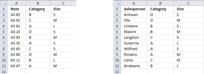
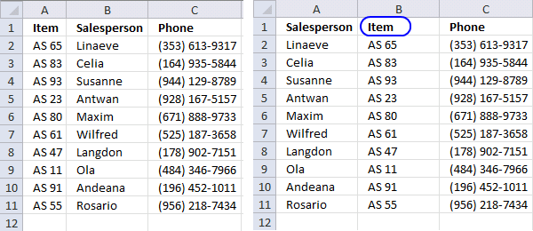
This example demonstrates how to match multiple values from two different columns, both values must match.
Below is the merged list. The COUNTIFS function allows you to match multiple columns simultaneously.
Array formula in cell D2:
This is an array formula and you need to enter this formula differently than a regular formula.
- Type the formula in cell D2.
- Press and hold CTRL + SHFT simultaneously.
- Then press ENTER once.
- Release all keys.
If you did it right, there are now curly brackets before and after the formula shown in the formula bar.
Copy cell D2 and paste it to D3:D11.
5.1 Explaining array formula in cell D2

The following link takes you to an explanation of how the "Evaluate Formula" tool works.
Step 1 - Check if value in cell B2 matches 'Ex 4 - Sheet2'!$B$2:$B$11 AND if value in cell C2 matches 'Ex 4 - Sheet2'!$C$2:$C$11
The COUNTIFS function allows you to use multiple arguments, in fact, up to 254 additional arguments.
It works just like the COUNTIF function meaning it counts the number of cells based on a condition, however, it also lets you use multiple criteria requiring you to enter the formula as an array formula.
COUNTIFS(criteria_range1, criteria1, [criteria_range2, criteria2]…)
We are going to use two conditions an compare them to two different columns, 1 equals True and 0 (zero) equals False. If both match on the same row the returned array returns 1 on the same relative position in the array.
COUNTIFS(B2,'Ex 4 - Sheet2'!$B$2:$B$11,C2,'Ex 4 - Sheet2'!$C$2:$C$11)
returns {0; 0; 1; 0; 0; 0; 0; 0; 0; 0}
Step 2 - Find the relative position of 1
The MATCH function looks for 1 in the array and returns a number representing the relative position in the array. It returns an error value if not found at all.
MATCH(lookup_value, lookup_array, [match_type])
MATCH(1,COUNTIFS(B2,'Ex 4 - Sheet2'!$B$2:$B$11,C2,'Ex 4 - Sheet2'!$C$2:$C$11),0)
becomes
MATCH(1,{0; 0; 1; ... ; 0},0)
and returns 3 meaning number 1 is in position 3 in the array.
Step 3 - Return a value of the cell at the intersection of a particular row and column
The INDEX function then returns the value on the same row from cell range A2:A11 using the result from the MATCH function.
INDEX(array, [row_num], [column_num])
INDEX('Ex 4 - Sheet2'!$A$2:$A$11, MATCH(1, COUNTIFS(B2, 'Ex 4 - Sheet2'!$B$2:$B$11, C2, 'Ex 4 - Sheet2'!$C$2:$C$11), 0))
returns "Linaeve" in cell D2.

6. Update list with new values if possible
Overview
Updating a list using copy/paste is a boring task. This blog article describes how to update values in a price list with new values.
Sheet 1 is the old price list. It contains 5000 products and amounts.

Sheet2 is the new price list. It contains 2000 random products from the old price list with new prices. (There are no new products)

6.1 How to create a new list with the latest prices.
Copy all products from sheet1 into sheet 3

Now let us find out if a new price exists.
Sheet3, formula in B2:

Double press with left mouse button on lower right corner of cell B2.

The formula is copied down to last adjacent product.
Sheet3, formula in C2:
Double press with left mouse button on lower right corner of cell C2 to copy the formula as far down as needed.

I created column B to make sure the values are the same as in sheet2 and to make it easier to understand the formula in cell C2.
6.2 Explaining the formula in cell C2
Step 1 - Find out if a new price exists
Match returns the relative position of an item in (Sheet2!$A$2:$A$2001) that matches a specified value (A2).
MATCH(A2, Sheet2!$A$2:$A$2001, 0) returns #N/A. This means "Product AT" can´t be found in sheet2.
ISERROR(MATCH(A2, Sheet2!$A$2:$A$2001, 0)) returns TRUE.
Step 2 - Identify sheet and price
The formula returned TRUE in cell C2. This means there is no new price. Let´s find the old price in sheet1 instead.
INDEX(Sheet1!$B$2:$B$5000, MATCH(A2, Sheet1!$A$2:$A$5000, 0))
MATCH(A2, Sheet1!$A$2:$A$5000, 0) returns 1. "Product AT" is found on the first row on sheet1.
INDEX(Sheet1!$B$2:$B$5000, 1) returns $43,90.
If formula in step 1 had returned False
If the formula had returned False in cell C2, we would need to look for the new price in sheet2.
INDEX(Sheet2!$B$2:$B$2001, MATCH(A2, Sheet2!$A$2:$A$2001, 0))
Get Excel Example File
automate_excel_pricelist.zip (300 KB)
Combine merge category
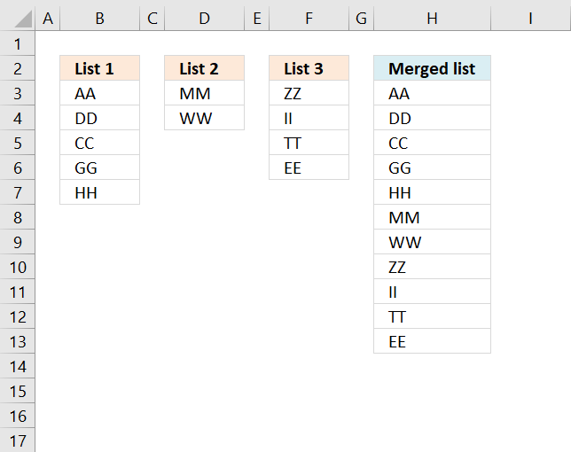
The above image demonstrates a formula that adds values in three different columns into one column. Table of Contents Merge […]
Excel categories
12 Responses to “Merge tables based on a condition”
Leave a Reply
How to comment
How to add a formula to your comment
<code>Insert your formula here.</code>
Convert less than and larger than signs
Use html character entities instead of less than and larger than signs.
< becomes < and > becomes >
How to add VBA code to your comment
[vb 1="vbnet" language=","]
Put your VBA code here.
[/vb]
How to add a picture to your comment:
Upload picture to postimage.org or imgur
Paste image link to your comment.
Hi,
Using the IFERROR in Excel 2007, you could use the formula below, whereby you do not need the Helper column B.
=IFERROR(VLOOKUP(A2, Sheet2!$A$2:$B$2001, 2, 0), VLOOKUP(Sheet3!A2, Sheet1!$A$2:$B$5000, 2, 0))
Why is it necessary to make the Formula an Array formula, it seems to work just fine witout it
Kanti Chiba,
you are right. It is not necessary to create an array formula.
Column B is not a helper column, it is created to make the formula in column C easier to understand.
Thanks for your contribution!
Thank you for this, especially for the last example, a really clever use of the COUNTIFS function.
I have to ask, how did you find out that COUNTIFS intially returns its result as an array? Been using it for so long, but I only learned that now.
Oh! You intentionally reversed criteria and criteria range. Sorry I missed that..
Patrick,
Thank you for this, especially for the last example, a really clever use of the COUNTIFS function.
Yes, most excel functions can return an array of values.
Thank you Mr. (Oscar)
On this wonderful business
Hi Oscar - You are amazing! I was hoping you might help me. I run a restaurant. I need to do a menu item comparison. Some of the items on my 2014 menu are the same as my 2013 menu, but I also have items from my 2013 menu that are not on 2014's menu. My spreadsheet has the following columns:
Menu
Item Name 2014 2013 2014 2013
Qty Sold Qty Sold Var Net Sales Net Sales Var
I have to run the 2014 report from my point-of sale first, and then the 2013 report second. Then I cut from the 2014 and 2013 reports and paste into the relative columns in the spreadsheet shown above. Because there are items on my 2014 menu that weren't on my 2013 menu, and items on my 2013 menu that weren't on my 2014 menu, when I get to one of those items, I'm constantly having to add rows -- its extremely time consuming. Can you help me with some sort of array formula that will sort this data for me? Thanks - John
Thank you for this article.
Suppose I have three sheets(Sheet1, Sheet2, Sheet3) containing the daily deposit in a bank with three different branches.
Sheet1
Brach 1
Sl. No Date Name Amount
1 4-May-14 A Banerjee 400
2 5-May-14 S Das 6000
3 2-Jun-14 Rajesh Mahato 4000
Sheet2
Brach 2
Sl. No Date Name Amount
1 23-May-14 Koushik Bag 20300
2 24-May-14 Tapan Roy 30000
3 8-Jun-14 Srikanto Koley 8900
Sheet3
Brach 3
Sl. No Date Name Amount
1 3-Apr-14 S Chandra 700
2 6-Jun-14 Pintu Basu 2000
I want to produce Sheet4 without using any macro.
Sheet4
Sl. No Date Name Amount
1 3-Apr-14 S Chandra 700
2 4-May-14 A Banerjee 400
3 5-May-14 S Das 6000
4 23-May-14 Koushik Bag 20300
5 24-May-14 Tapan Roy 30000
6 2-Jun-14 Rajesh Mahato 4000
7 6-Jun-14 Pintu Basu 2000
8 8-Jun-14 Srikanto Koley 8900
Can it be possible?
Please help.
if you have a price list for products and you want to update that from a new price list the below formula may help
=IFERROR(INDEX($H$2:$I$4, MATCH(A2, $H$2:$H$4,0), 2),B2)
Hi, what if there is some new products in the new price list. And what I want to do is to identify the "values" of these product, so I know the codes of the new products. Can we do that?
how do I create a list based on cell values. I have 2 or more series (pic1) and pic2 is the list I want excel to produce.
(pic1) https://s23.postimg.org/ny600047v/Screen_Shot_2016_02_09_at_7_01_21_PM.png
(pic2) https://s23.postimg.org/44tw7aqu3/Screen_Shot_2016_02_09_at_7_01_31_PM.png
In the scenario above, I must make a book consisting of 3 sections: A (20 pages), B (12 pages) and C (8 pages). C pages go into B section, and these go into A section. The number of section changes and the number of pages of a section changes.
How do I get excel to automatically produce a list (similar to pic2) based on values input in pic1?
1. Create one column and do a VLOOKUP for your price in your 'new price sheet;
2. create a second column with the code: 'IFNA'
if your price sheet has #NA select the cell with new price, if it has a value from the old sheet basically its NOT #n/a ; and Excel will keep the old price.
suppose you have an old price in the Cell?
you can create a third column, use your new price sheet and turn all prices in your master sheet to the text '#N/A' then do steps 1 & 2.
Granted this is a 3 column, 3 step process,
But the time and grief saved creating a single formula solution that actually works in the end is priceless.
and you can create a Macro to do this.