How to use the HOUR function

What is the HOUR function?
The HOUR function returns an integer representing the hour of an Excel time value. The returning number is ranging from 0 (12:00 A.M.) to 23 (11:00 P.M.).
Table of Contents
1. Introduction
1. What is an integer?
An integer is a whole number that can be positive, negative, or zero, but not a fraction or decimal. Excel can't calculate the hour based on negative integers.
What is an Excel time value?
Excel time is actually a decimal number ranging between 0 and 1 in Excel and then formatted as time.
For example, 12:00 PM is represented as 0.5 because it is half of a day, you can verify this by typing 12:00 PM in a cell and then change the cell formatting to general. This will show the value as Excel interprets it.
How does Excel recognize time values?
Excel recognizes certain text strings like "6:45 PM" as valid time values. A recognized time value is right aligned in the cell just like a regular number, shown in the image below in cell B2.

A time number that is not recognized is left aligned which is demonstrated in cell B4 in the image above. This visual feedback lets you easily spot values that need closer inspection.
What is an hour in an Excel time value?

1/24 or approx. 0.04166667 represents one hour in Excel time value. Excel uses a number 0 <= x <= 1 in decimal form to represent time in a worksheet. 0 is zero hours and 1 is 24 hours. To get one hour we must divide 1 by 24 and we get 1/24.
Why is 1 equal to 24 hours?
This has to do how Excel handles dates. Each date is represented by an integer and one day is 1 in Excel.
Dates are stored numerically but formatted to display in human-readable date/time formats, this enables Excel to do work with dates in calculations.

For example, dates are stored as sequential serial numbers with 1 being January 1, 1900 by default. The integer part (whole number) represents the date the decimal part represents the time.
This allows dates to easily be formatted to display in many date/time formats like mm/dd/yyyy, dd/mm/yyyy and so on and still be part of calculations as long as the date is stored numerically in a cell.
You can try this yourself, type 10000 in a cell, press CTRL + 1 and change the cell's formatting to date, press with left mouse button on OK. The cell now shows 5/18/1927.
What is the decimal form?
The decimal form or decimal number system represents values using digits 0-9 and a decimal point. Each digit position represents a power of 10 - units, tens, hundreds, etc. The decimal point separates the integer part from the fractional part. Decimal values allow representation of fractional numbers in a standard notation.
Where is AM/PM used?
AM/PM is used in the United States, Canada, Mexico, Australia, United Kingdom and a few other countries. AM refers to times from midnight to noon. PM refers to times from noon to midnight.
Where is the 24 hour clock used?
The 24 hour clock is used in continental Europe including Scandinavia, China, India and most countries except those above. Used in formal documents like schedules, timetables, business contracts. Used by scientists, aviation, hospitals, transportation services, military. Avoids AM/PM ambiguity and potential confusion.
| AM/PM | 24 hour clock |
| 12:00 AM | 0:00 |
| 1:00 AM | 1:00 |
| 2:00 AM | 2:00 |
| 3:00 AM | 3:00 |
| 4:00 AM | 4:00 |
| 5:00 AM | 5:00 |
| 6:00 AM | 6:00 |
| 7:00 AM | 7:00 |
| 8:00 AM | 8:00 |
| 9:00 AM | 9:00 |
| 10:00 AM | 10:00 |
| 11:00 AM | 11:00 |
| 12:00 PM | 12:00 |
| 1:00 PM | 13:00 |
| 2:00 PM | 14:00 |
| 3:00 PM | 15:00 |
| 4:00 PM | 16:00 |
| 5:00 PM | 17:00 |
| 6:00 PM | 18:00 |
| 7:00 PM | 19:00 |
| 8:00 PM | 20:00 |
| 9:00 PM | 21:00 |
| 10:00 PM | 22:00 |
| 11:00 PM | 23:00 |
| 12:00 AM | 0:00 |
2. Syntax
HOUR(serial_number)
3. Arguments
| serial_number | Required. An Excel time value that you want to calculate the hour of. |
4. Example
This example demonstrates the HOUR function in cell C3, it extracts the hour from the Excel time value specified in cell B3: "1:34:22 PM"
Formula in cell C3:
1:00 PM represents the 13th hour.
5. HOUR function not working

The HOUR function returns
- #NUM! error if the decimal is a negative value.
- #VALUE! error if the Excel time value is invalid.
5.1 Troubleshooting the error value
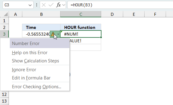
When you encounter an error value in a cell a warning symbol appears, displayed in the image above. Press with mouse on it to see a pop-up menu that lets you get more information about the error.
- The first line describes the error if you press with left mouse button on it.
- The second line opens a pane that explains the error in greater detail.
- The third line takes you to the "Evaluate Formula" tool, a dialog box appears allowing you to examine the formula in greater detail.
- This line lets you ignore the error value meaning the warning icon disappears, however, the error is still in the cell.
- The fifth line lets you edit the formula in the Formula bar.
- The sixth line opens the Excel settings so you can adjust the Error Checking Options.
Here are a few of the most common Excel errors you may encounter.
#NULL error - This error occurs most often if you by mistake use a space character in a formula where it shouldn't be. Excel interprets a space character as an intersection operator. If the ranges don't intersect an #NULL error is returned. The #NULL! error occurs when a formula attempts to calculate the intersection of two ranges that do not actually intersect. This can happen when the wrong range operator is used in the formula, or when the intersection operator (represented by a space character) is used between two ranges that do not overlap. To fix this error double check that the ranges referenced in the formula that use the intersection operator actually have cells in common.
#SPILL error - The #SPILL! error occurs only in version Excel 365 and is caused by a dynamic array being to large, meaning there are cells below and/or to the right that are not empty. This prevents the dynamic array formula expanding into new empty cells.
#DIV/0 error - This error happens if you try to divide a number by 0 (zero) or a value that equates to zero which is not possible mathematically.
#VALUE error - The #VALUE error occurs when a formula has a value that is of the wrong data type. Such as text where a number is expected or when dates are evaluated as text.
#REF error - The #REF error happens when a cell reference is invalid. This can happen if a cell is deleted that is referenced by a formula.
#NAME error - The #NAME error happens if you misspelled a function or a named range.
#NUM error - The #NUM error shows up when you try to use invalid numeric values in formulas, like square root of a negative number.
#N/A error - The #N/A error happens when a value is not available for a formula or found in a given cell range, for example in the VLOOKUP or MATCH functions.
#GETTING_DATA error - The #GETTING_DATA error shows while external sources are loading, this can indicate a delay in fetching the data or that the external source is unavailable right now.
5.2 The formula returns an unexpected value
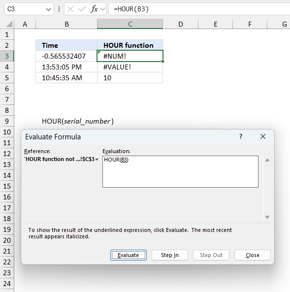
To understand why a formula returns an unexpected value we need to examine the calculations steps in detail. Luckily, Excel has a tool that is really handy in these situations. Here is how to troubleshoot a formula:
- Select the cell containing the formula you want to examine in detail.
- Go to tab “Formulas” on the ribbon.
- Press with left mouse button on "Evaluate Formula" button. A dialog box appears.
The formula appears in a white field inside the dialog box. Underlined expressions are calculations being processed in the next step. The italicized expression is the most recent result. The buttons at the bottom of the dialog box allows you to evaluate the formula in smaller calculations which you control. - Press with left mouse button on the "Evaluate" button located at the bottom of the dialog box to process the underlined expression.
- Repeat pressing the "Evaluate" button until you have seen all calculations step by step. This allows you to examine the formula in greater detail and hopefully find the culprit.
- Press "Close" button to dismiss the dialog box.
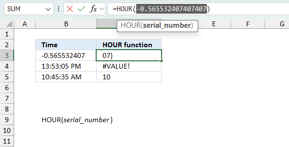
There is also another way to debug formulas using the function key F9. F9 is especially useful if you have a feeling that a specific part of the formula is the issue, this makes it faster than the "Evaluate Formula" tool since you don't need to go through all calculations to find the issue..
- Enter Edit mode: Double-press with left mouse button on the cell or press F2 to enter Edit mode for the formula.
- Select part of the formula: Highlight the specific part of the formula you want to evaluate. You can select and evaluate any part of the formula that could work as a standalone formula.
- Press F9: This will calculate and display the result of just that selected portion.
- Evaluate step-by-step: You can select and evaluate different parts of the formula to see intermediate results.
- Check for errors: This allows you to pinpoint which part of a complex formula may be causing an error.
The image above shows cell reference B3 converted to hard-coded value using the F9 key. The HOUR function requires numerical values larger than or equal to 0 (zero) which is not the case in this example. We have found what is wrong with the formula.
Tips!
- View actual values: Selecting a cell reference and pressing F9 will show the actual values in those cells.
- Exit safely: Press Esc to exit Edit mode without changing the formula. Don't press Enter, as that would replace the formula part with the calculated value.
- Full recalculation: Pressing F9 outside of Edit mode will recalculate all formulas in the workbook.
Remember to be careful not to accidentally overwrite parts of your formula when using F9. Always exit with Esc rather than Enter to preserve the original formula. However, if you make a mistake overwriting the formula it is not the end of the world. You can “undo” the action by pressing keyboard shortcut keys CTRL + z or pressing the “Undo” button
5.3 Other errors
Floating-point arithmetic may give inaccurate results in Excel - Article
Floating-point errors are usually very small, often beyond the 15th decimal place, and in most cases don't affect calculations significantly.
6. Alternative - cell formatting

You also have the option to format a cell containing an Excel time value so it shows only the hour part. Here is how:
- Select the cell.
- Press CTRL + 1 to open the "Format Cells" dialog box.
- Select category: Custom
- Create a new type: hh
- Press the "OK" button.
The image above shows cell B3 containing the following time value "1:34:22 PM", cell C3 references that value. This means that cell C3 contains the same value, however, cell formatting is applied which makes it show only the hour part.
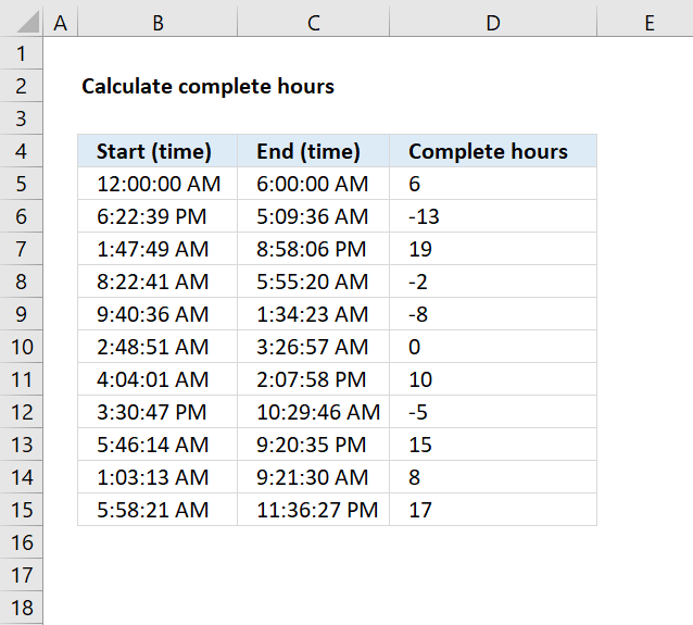
7. Count complete hours between two time values
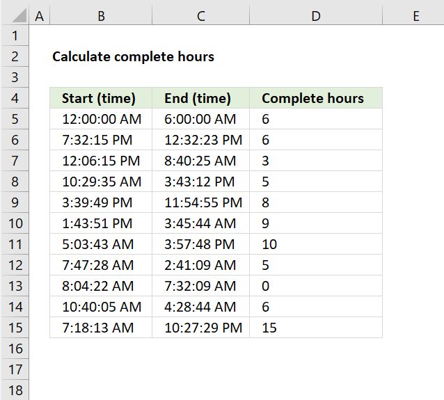
The formula in cell D5 calculates the number of complete hours between the time entries in cell B5 and C5.
Formula in cell D5:
Note that this formula works only with time entries, not date and time entries. It doesn't matter if the start time is past the end time, the formula will regardless return a positive hour value.
Explaining formula in cell D5
Step 1 - Subtract time entries
C5-B5
becomes
6:00:00 AM - 12:00:00 AM
Time entries in excel are actually a decimal value between 0 (zero) and 1. One hour is 1/24, six hours is 6/24 and so on.
0.25 - 0 equals 0.25
Step 2 - Remove sign
The ABS function removes the minus sign if it exists, the HOUR function can't calculate negative values.
ABS(C5-B5)
becomes
ABS(0.25) and returns 0.25.
Step 3 - Convert decimal to hour(s)
The HOUR function calculates hours based on a decimal value.
HOUR(ABS(C5-B5))
becomes
HOUR(0.25)
and returns 6.
The image above demonstrates a formula the returns negative hours if the start time is later than the end time.
Formula in cell D5:
Explaining formula in cell D5
This part of the formula HOUR(ABS(C5-B5)) is explained above.
Step 1 - Calculate if end date is smaller than the start date
C5<B5
becomes
0.25<0
and returns FALSE.
Step 2 - Return -1 if TRUE and 1 if FALSE
IF(C5<B5,-1,1)
becomes
IF(0.25<0,-1,1)
becomes
IF(FALSE,-1,1) and returns 1.
Step 3 - Multiply with result
HOUR(ABS(C5-B5))*IF(C5<B5,-1,1)
becomes
6*IF(C5<B5,-1,1)
becomes
6*1 and returns 6 in cell D5.
8. Count complete hours between two date and time values
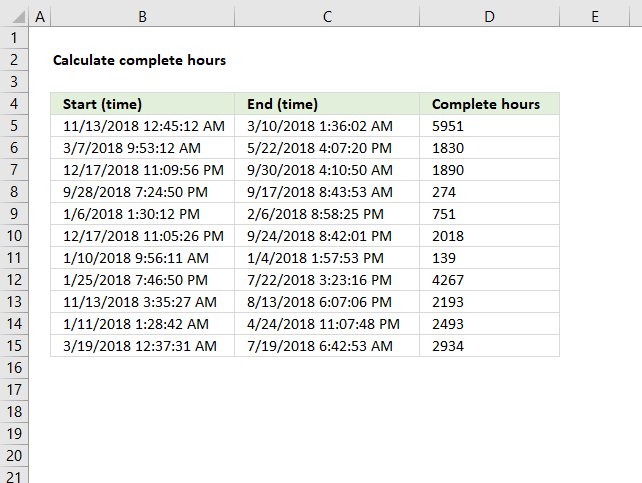
The picture above shows a formula that calculates complete hours between date and time entries.
Formula in cell D5:
If you want negative hours then remove the ABS function:
The TEXT function formats the result of C5-B5 into complete hours.
'HOUR' function examples
Functions in 'Date and Time' category
The HOUR function function is one of 22 functions in the 'Date and Time' category.
How to comment
How to add a formula to your comment
<code>Insert your formula here.</code>
Convert less than and larger than signs
Use html character entities instead of less than and larger than signs.
< becomes < and > becomes >
How to add VBA code to your comment
[vb 1="vbnet" language=","]
Put your VBA code here.
[/vb]
How to add a picture to your comment:
Upload picture to postimage.org or imgur
Paste image link to your comment.
Contact Oscar
You can contact me through this contact form