Create number series

Excel has a great built-in tool for creating number series named Autofill. The tool is great, however, in some situations, you need to rely on formulas.

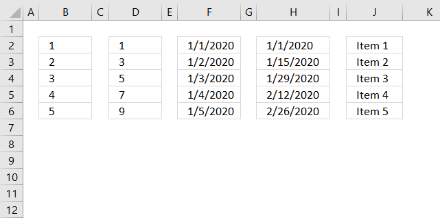
The Autofill is also able to create date series and values containing both text and numbers, shown in columns F, H and J above.

1. Where is the Autofill button on the ribbon?

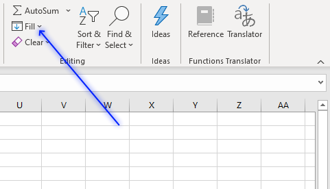
The Autofill button is located on tab "Home" on the ribbon. Press with left mouse button on the "Fill" button and a pop-up menu appears.

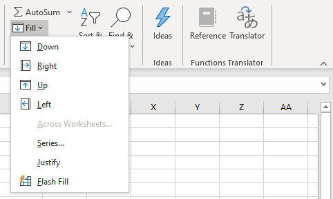
The pop-up menu shows:

• Down
• Right
• Up
• Left
• Across Worksheets...
• Series...
• Justify
• Flash Fill

You can also create a number series using the dot in the lower right corner of the selected cell.

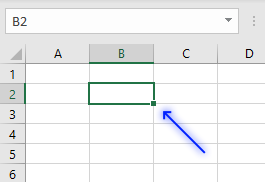
The two first examples below demonstrate how to use the dot to create a series of numbers.

Back to top

1.1 How to create a number series from 1 to n

The following two examples show you how to create a number sequence using two different techniques. The Autofill feature allows you to quickly create a series of numbers.

Example 1

The animated image above shows how to create a number sequence from 1 to 5. You can create a much larger series

1. Type 1 in cell B2.
2. Press Enter.
3. Press with right mouse button on on the black dot and drag down as far as needed.
   A pop-up menu appears.
4. Press with left mouse button on "Fill series".

Back to top

Example 2

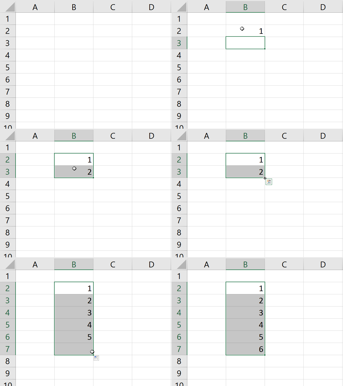
1. Type 1 in cell A3 and 2 in cell A4
2. Select A3 and A4
3. Press and hold with left mouse button on the black dot and drag down as far as needed.

Back to top

Example 3,

If you prefer a formula, try this one out:

The image above shows the formula entered in cell B2. Copy cell B2 and paste to cells below as far as needed.

The formula works as intended even if you insert rows above the cell B2.

Back to top

1.2 How to create a number series with every other number

The image above shows a list with every other number starting from 1 to n, in column D. To create this list follow these steps:

1. Select cell D2.
2. Type 1 and then press Enter.
3. Select cell D3 if it is not already selected.
4. Type 3 and press Enter on your keyboard.
5. Select cell range D2:D3.
6. Press and hold with left mouse button on the dot in the lower right corner of the selected cell range.
7. Drag with mouse downwards as far as needed.
8. Release left mouse button.

Back to top

1.3 How to create a series of dates

Column F in the image above shows a date series from 1/1/2020 to 1/5/2020. Here is how to quickly create it:

1. Select cell F2.
2. Type 1/1/2020 and then press Enter on your keyboard.
3. Select cell F2 again.
4. Press and hold with right mouse button on the dot located in the lower right corner of the select cell, in this case, cell F2.
5. Drag with mouse downwards as far as needed.
6. Release right mouse button.
7. A pop-up menu appears.
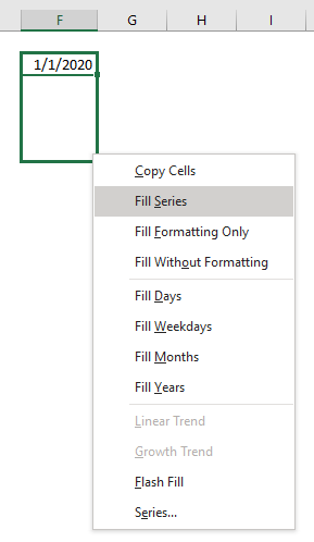
8. Press with left mouse button on "Fill Series".

Back to top

1.4 How to create a series of dates based on a given period

Column H shows a date series based on every other week or 14 days.

1. Select cell H2.
2. Type 1/1/2020 or the start date you want to use, and then press Enter.
3. Select cell H3 if it is not already selected.
4. Type 1/15/2020 or the date you want to use, and press Enter on your keyboard.
   The Autofill tool will use the difference in days between the first date (H2) and the second date (H3) to create the remaining dates.
5. Select cell range H2:H3.
6. Press and hold with left mouse button on the dot located in the lower right corner of the selected cell range.
7. Drag with mouse to cells below as far as needed.
8. Release left mouse button.

Back to top

1.5 How to create a a series of values based on text and numbers

The Autofill tool allows you to use values containing both text and numbers as well. Column J shows this in the image above.

1. Select cell J2.
2. Type Item 1
3. Select cell J2 again.
4. Press and hold with left mouse button on the dot located in the lower right corner of the selected cell.
5. Drag with mouse to cells below as far as needed.

Back to top

2. Create a repeating number sequence using a formula

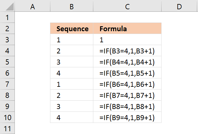
In this example, I am going to create a repeating number sequence 1, 2, 3, 4.

This formula checks if the previous sequence number is 4, if true it restarts with value 1. If false it adds the previous sequence number with 1.

Select cell B3 and type 1. Then press Enter.

Formula in B4:

Type above formula in cell B4. Press Enter. Note, you don't need to enter all the formulas in cell range B2:B10. Only the number in cell B3 and the formula in cell B4.

Back to top

Explaining formula in cell B4

The IF function allows you to control the outcome based on a condition or multiple conditions, in other words, it returns one value if the logical test is TRUE and another value if the logical test is FALSE.

It contains three parts, logical expression, value to return if the logical expression evaluates to true, and another value to return if the logical expression evaluates to false.

IF(logical_test, [value_if_true], [value_if_false])

Step 1 - Logical expression

B3=4

B3 is a relative cell reference, relative meaning it changes when the cell is copied and then pasted to another cell, in this case, the adjacent cell below.

For example, cell reference B3 changes to cell B4 when cell B4 is copied to cell B5.

Remember that this formula is in cell B4 so a cell reference to cell B3 is the adjacent cell above. B3 is 1.

B3=4 returns boolean value FALSE. This value determines if the second argument or third argument will be evaluated next.

Recommended articles

Step 2 - Next argument

IF(B3=4, 1, B3+1) returns 2 in cell B4.

The logical expression returns FALSE, this means that the third argument will now be calculated.

Next cells

It is not until cell B7 something unexpected happens. The logical expression now evaluates to TRUE.

IF(B6=4, 1, B6+1) returns 1.

This will make the IF function calculate the second argument instead of the third as before.

IF(logical_test, [value_if_true], [value_if_false])

The series starts all over again beginning with 1.

Back to top

3. Create a number series and restart when a cell value equals a given condition

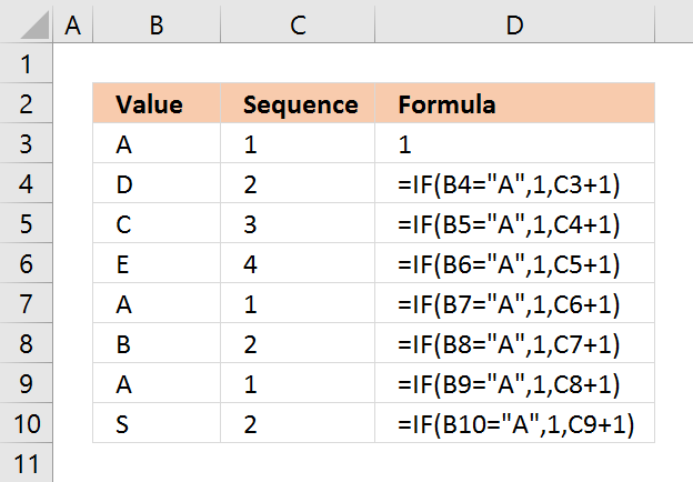
In this example, the number sequence restarts every time the adjacent cell value in column B is equal to "A".

Select cell C3 and type 1. Then press Enter.

Formula in C4:

Copy cell C4 and paste to cells below as far as needed.

Back to top

Explaining formula in cell C4

The IF function returns one value if the logical test is TRUE and another value if the logical test is FALSE.

IF(logical_test, [value_if_true], [value_if_false])

Step 1 - Calculate logical expression

The logical expression is the first argument, in this case: B4="A". Cell reference B4 is a relative cell reference, it changes when the cell is copied to cells below. Note, you need to copy the cell not the formula for this to work.

The text string "A" is the condition, if cell B4 is equal to the condition it returns TRUE, otherwise FALSE. TRUE and FALSE are boolean values in Excel.

B4="A" returns FALSE.

Step 2 - Return second argument if TRUE and third argument if FALSE.

The second argument is 1 and the third argument adds 1 to the number in cell C3.

IF(B4="A",1,C3+1) returns 2 in cell C4.

Next cells

It is not until cell C7 things change in the formula.

IF(B7="A",1,C6+1) returns 1. The series now start all over with number 1.

Back to top

4. Create a number sequence to count records by year and month (sorted list)

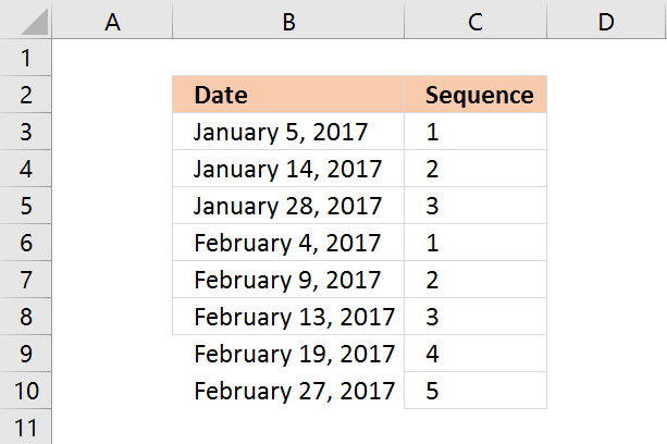
This formula checks if the previous date has the same year and month as the current cell date. If true the previous sequence number is added by 1. If false the sequence starts all over again with 1.

The following formula will only work if the dates in column B are sorted from earliest to latest.

Formula in C4:

Copy cell C4 and paste to cells below as far as necessary.

Back to top

Explaining formula in cell C4

Step 1 - Convert dates to month and year

TEXT(B4, "M-YYYY")

Step 2 - Compare values

TEXT(B4, "M-YYYY")=TEXT(B3, "M-YYYY")

IF(logical_test, [value_if_true], [value_if_false])

Step 3 - If function returns one value if True and another value if False

IF(TEXT(B4, "M-YYYY")=TEXT(B3, "M-YYYY"), C3+1, 1)

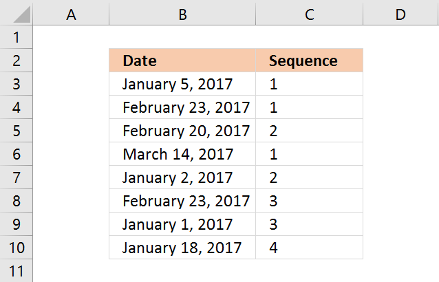
5. Create a number sequence to count records based on year and month (unsorted list)

Array formula in  B32:

Copy cell C3 and paste to cells below as far as necessary.

Recommended articles

Back to top

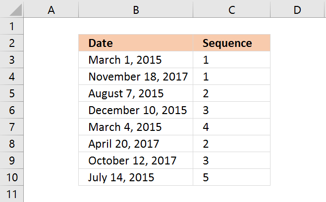
6. Create a number sequence to count dates based on year

This formula works fine with both sorted and unsorted lists. It simply counts the current cell year in the previous years cell range.

Formula in B39:

Copy cell C3 and paste to cells below as far as necessary.

Back to top

7. Create a number sequence to count individual products

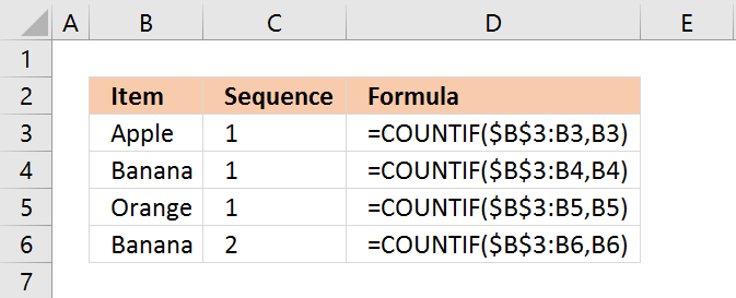
The COUNTIF function simply counts how many times the Item value has been displayed.

Formula in C3:

The first argument has a cell range that expands when you copy the cell to cells below.

Copy cell C3 and paste to cells below as far as necessary.

Recommended articles

Back to top

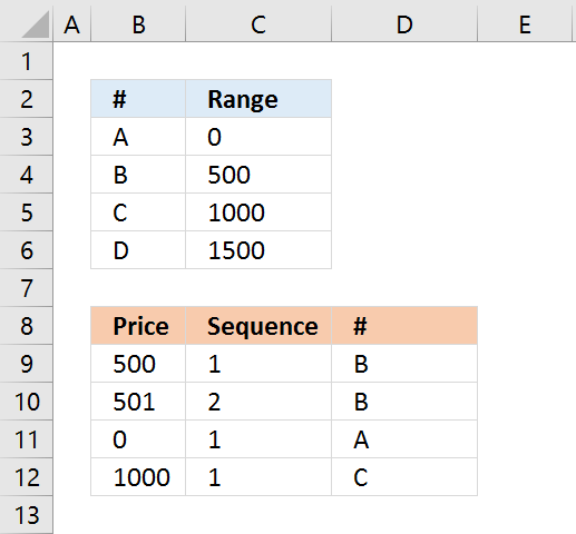
8. Create a number sequence to count prices within specific ranges

The formula in cell C9 creates a sequence depending on which range the price is in.

Formula in C9:

Copy cell C9 and paste to cells below as far as necessary.

Back to top

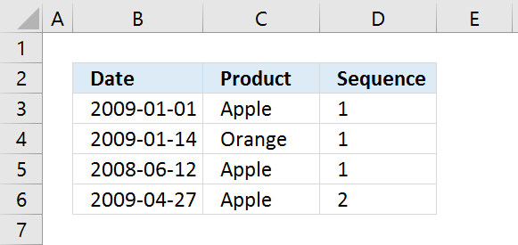
9. Create a number sequence to count records by individual products and years

Formula in D3:

Copy cell D3 and paste to cells below as far as needed.

Back to top

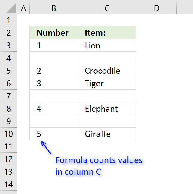
10. Create a numbered list ignoring blank cells

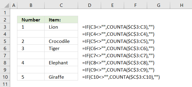
The formula in column B returns a running count based on values in column C.

Formula in cell B3:

The formula consists of two Excel functions. The IF function checks if the corresponding value in column C is not empty.

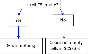If cell C3 is not empty the COUNTA function counts the number of cells in cell range $C$3:C3 that are not empty.

Cell range $C$3:C3 has one cell that is not empty so the formula returns 1 in cell B3.

Note that cell reference $C$3:C3 expands when you copy cell B3 and paste to cells below.

For example, in cell B4 the cell reference changes to $C$3:C4.

If cell C3 is empty the formula returns nothing.

Watch a video where I demonstrate the techniques described below

Back to top

Sequence category

More than 1300 Excel formulas

Excel categories

Comments (12)