Repeat values across cells

Table of Contents
1. Repeat values across cells
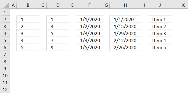
This article explains how to repeat specific values based on a table, the table contains the items to be repeated and how many times they will be repeated.
The array formula in cell A6 utilizes the table and repeats the values until the condition is met.
There is also a section below that explains how to repeat values in sequence based on corresponding numbers.
I failed to find the right article in your blog and therefore I want to ask you in newest post. So I have a table similar to this:
A 5
B 2
C 1
D 4
Is it possible with a formula to generate a list like this:
A
A
A
A
A
B
B
C
D
D
D
D
Thank you in advance!
Array formula in cell A6:
How to create an array formula
- Double press with left mouse button on cell A6 so the prompt appears.
- Copy and paste the array formula above to the cell.
- Press and hold CTRL + SHIFT simultaneously.
- Press Enter once.
- Release all keys.
You can check using the formula bar that you did above steps right, Excel tells you if a cell contains an array formula by surrounding the formula with a beginning and ending curly brackets, like this: {=array_formula}.
Don't enter these characters yourself they show up automatically if you did the above steps correctly.
Explaining array formula in cell A6

I recommend that you use the built-in "Evaluate Formula" feature in Excel to better understand and troubleshoot formulas, it is a great tool that allows you to see each calculation step.
Go to tab "Formulas" on the ribbon, then press with left mouse button on "Evaluate Formula" button. Press with left mouse button on "Evaluate" button to move to next calculation step, press with left mouse button on "Close" button to dismiss the dialog box.
Step 1 - Count previous values
The COUNTIF function counts values in a cell range based on a condition, however, in this case, I use a growing cell reference that expands when you copy the cell and paste to cells below.
This will make the COUNTIF function count based on multiple conditions, this technique is what makes you required to enter the formula as an array formula.
This way the function keeps track of previous values above the current cell so the correct number of values is returned based on the table.
COUNTIF($A$5:A5,$A$1:$A$4)
COUNTIF(range, criteria)
The first argument is $A$5:A5 which is a cell reference, however, it contains two parts. The first part is an absolute cell reference pointing to A5, you can tell that it is absolute by the $ characters.
It means that the cell reference is locked to cell A5, both the column and row number is, locked, and does not change when you copy the cell to cells below. There are exceptions to this like inserting new rows or columns.
The second part is a relative cell reference and this changes when you copy the cell and paste to cells below which is great because the cell reference expands and takes multiple cells into account.
For example, in cell A6 the cell reference is $A$5:A5, however, in cell A7 the cell reference changes to $A$5:A6 and this makes the formula aware of previous returned values above the current cell.
COUNTIF($A$5:A5,$A$1:$A$4)
becomes
COUNTIF("",{"A";"B";"C";"D"})
and returns {0;0;0;0}
In cell A6 there are no previous values above, only cell A5 which is empty.
The COUNTIF function returns an array containing the same number of values as the table and each value in the array represents how many times the values in the table have been displayed.
An array uses commas and semicolons to separate values, commas are between columns and semicolons are between rows.
Step 2 - Compare array values to list
This step checks if the values in the array is equal to the numbers in the table, this works because the values in the array correspond to the numbers in the table.
The equal sign compares the returned values from the COUNTIF function with the values in cell range B1:B4 and returns TRUE or FALSE. Note that the cell reference to B1:B4 is absolute. We don't want it to change when the cell is copied to cells below.
COUNTIF($A$5:A5,$A$1:$A$4)=$B$1:$B$4
becomes
{0;0;0;0}={5;2;1;4}
and returns {FALSE;FALSE;FALSE;FALSE}
Not a single value meets the criteria in the table in cell A6, that is why all values in the array are FALSE.
Step 3 - Match first FALSE value in array
The MATCH function returns the position of a given value in a cell range or array.
MATCH(lookup_value, lookup_array, [match_type])
The first argument is FALSE, we want to know the position of the first value that has not been repeated the number of times specified in the table.
The second argument is the array we created in step 2 and the third argument is 0 (zero) which means we want an exact match.
MATCH(FALSE, COUNTIF($A$5:A5,$A$1:$A$4)=$B$1:$B$4,0)
becomes
MATCH(FALSE, {FALSE;FALSE;FALSE;FALSE},0)
and returns 1.
Step 4 - Return a value of the cell at the intersection of a particular row and column
The INDEX function returns a value from a cell range or array based on a row and column number. The column number is optional if the cell range is only a single column.
INDEX($A$1:$A$4, MATCH(FALSE, COUNTIF($A$5:A5, $A$1:$A$4)=$B$1:$B$4, 0))
becomes
=INDEX($A$1:$A$4, 1)
and returns A in cell A6.
Repeat values in a predetermined series
This example demonstrates a formula that repeats values in a given sequence and also how many times each value is to be repeated.
Hi Oscar,
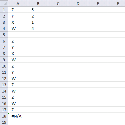
Great Job.. Is this possible to repeat the range according to criteria in loop.. like below.Z 5
Y 2
X 1
W 4then Z 5 Times, Y 2 Times.... but in series
Z
Y
X
W
Z
Y
W
Z
W
Z
W
ZRegards,
Deb
Array formula in cell A6:
Explaining formula in cell A6
Step 1 - Count previous values
COUNTIF($A$5:A5, $A$1:$A$4)=$B$1:$B$4
becomes
{0;0;0;0}=$B$1:$B$4
becomes
{0;0;0;0}={5;2;1;4}
and returns
{FALSE;FALSE;FALSE;FALSE}.
Step 2 - Replace values to be repeated with their count
IF(COUNTIF($A$5:A5, $A$1:$A$4)=$B$1:$B$4, "", COUNTIF($A$5:A5, $A$1:$A$4))
becomes
IF({FALSE; FALSE; FALSE; FALSE}, "", {0;0;0;0})
and returns
{0;0;0;0}.
Step 3 - Find smallest count number
MIN(IF(COUNTIF($A$5:A5, $A$1:$A$4)=$B$1:$B$4, "", COUNTIF($A$5:A5, $A$1:$A$4)))
becomes
MIN({0;0;0;0})
and returns 0 (zero).
Step 4 - Find relative position
MATCH(MIN(IF(COUNTIF($A$5:A5, $A$1:$A$4)=$B$1:$B$4, "", COUNTIF($A$5:A5, $A$1:$A$4))), IF(COUNTIF($A$5:A5, $A$1:$A$4)=$B$1:$B$4, "", COUNTIF($A$5:A5, $A$1:$A$4)), 0)
becomes
MATCH(0, IF(COUNTIF($A$5:A5, $A$1:$A$4)=$B$1:$B$4, "", COUNTIF($A$5:A5, $A$1:$A$4)), 0)
becomes
MATCH(0, {0;0;0;0}, 0)
and returns 1.
Step 5 - Return value based on position
INDEX($A$1:$A$4, MATCH(MIN(IF(COUNTIF($A$5:A5, $A$1:$A$4)=$B$1:$B$4, "", COUNTIF($A$5:A5, $A$1:$A$4))), IF(COUNTIF($A$5:A5, $A$1:$A$4)=$B$1:$B$4, "", COUNTIF($A$5:A5, $A$1:$A$4)), 0))
becomes
INDEX($A$1:$A$4, 1)
and returns "Z" in cell A6.
3. Find the most/least consecutive repeated value - VBA
This post Find the longest/smallest consecutive sequence of a value has a few really big array formulas. Today I would like to show you how to build a simple UDF that will simplify these formulas significantly.
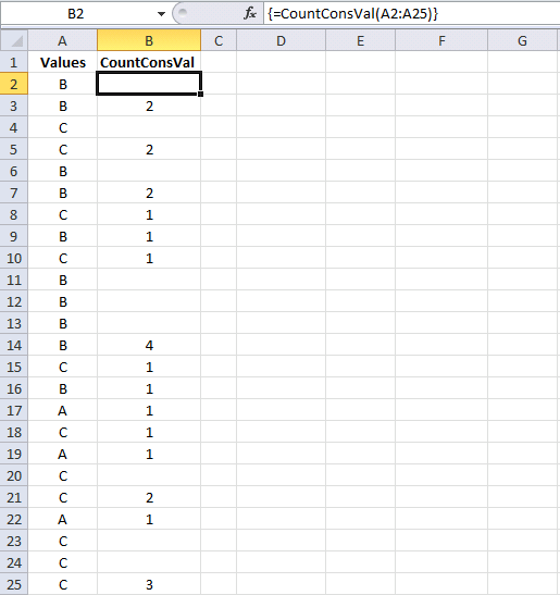
The following user-defined function returns the size of each consecutive sequence in a range. The udf is entered in cell range B2:B25, see this picture.
The UDF returns an array with the same size as the argument range. The cell range has 24 cells and the array has 24 values.
3.1. VBA code
'Name User Defined Function
Function CountConsVal(r As Range)

'Dimension variables and declare data types
Dim i As Long, s As Long

'Save value in cell range r to variable Rng
Rng = r.Value

'Iterate through values in array variable Rng
For i = LBound(Rng, 1) To UBound(Rng, 1) - 1

    'Check if next value is equal to current value
    If Rng(i, 1) = Rng(i + 1, 1) Then

        'Add 1 to numbers stored in variable s
        s = s + 1

        'Clear container in array variable Rng
        Rng(i, 1) = ""

    'Go here if next value is NOT equal to current value
    Else

        'Add 1 to variable s and save to container in array variable Rng
        Rng(i, 1) = s + 1

        'Save 0 to variable s
        s = 0
    End If
Next i

'Add 1 to variable s and then save result to the last container in array variable Rng
Rng(UBound(Rng), 1) = s + 1

'Return values to worksheet
CountConsVal = Rng
End Function
3.2. Array formulas
Array formula in cell E3:
Array formula in cell E4:
Array formula in cell G3:
Array formula in cell G4:
Array formula in cell E7:
Array formula in cell E8:
3.3. Where to put the code?
To build a user-defined function in your workbook, follow these steps:
- Press Alt + F11 to open the visual basic editor.
- Press with left mouse button on "Insert" on the menu.
- Press with left mouse button on "Module".
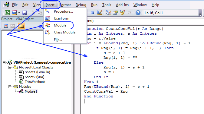
- Copy the code above and paste it to the code module.
3.4. Explaining the User Defined Function
3.4.1 Function name and arguments
A user-defined function procedure always starts with "Function" and then a name. This UDF has a single argument r. Variable r is a range.
Function CountConsVal(r As Range)
3.4.2 Declaring variables
Variable i and s are declared data type Long. Read more about Defining data types.
Dim i As Long, s As Long
3.4.3 Transfer values from r (range) to a Rng (variant) array
Rng = r.Value
3.4.4 For ... Next statement
Repeats a group of statements a specified number of times. LBound returns the lower bound of an array and UBound the upper bound.
LBound(array, dimension) UBound(array, dimension), the dimension argument can be omitted if the array is a one-dimensional array. In this case the Variant Rng is a two-dimensional array despite the fact that the range r is a one-dimensional array. UBound(Rng, 1) returns the number of rows in Rng array.
For i = LBound(Rng, 1) To UBound(Rng, 1) - 1

...

Next i
3.4.5 If ... then... Else ... End If
Check if the current value (i) is equal to the next value (i+1)
If Rng(i, 1) = Rng(i + 1, 1) Then
3.4.6 Add number 1 to variable s
s = s + 1
3.4.7 Delete value in array
Rng(i, 1) = ""
3.4.8 Assign a value (s + 1) to array variable Rng(i, 1)
The current value in the array is equal to s + 1
Rng(i, 1) = s + 1
3.4.9 Assign 0 (zero) to variable s
s = 0
3.4.10 Assign a value (s + 1) to the last value in the array Rng(UBound(Rng), 1)
Rng(UBound(Rng), 1) = s + 1
3.4.11 The udf returns an array of values
CountConsVal = Rng
3.4.12 End a udf
A function procedure ends with this statement.
End Function
4. How to count repeating values

This article demonstrates ways to count contiguous values in a column, in other words, values that repeat and are adjacent.
4.1. How to count any contiguous value
The formula in cell D4 checks if the value in cell D3 is not equal to the value in cell D4. If true (not equal) the result is 1. If false (equal) the formula adds 1 to the previous value above.
Copy cell D4 and paste to cells below as far as needed in order to count all values in column B.
Formula in cell D4:
The formula in cell F3 simply extracts the largest number from cell range D3:D14. Adjust cell ref D3:D14 if you have more values than the example shown in the image above.
Formula in cell F3:
Explaining formula in cell D4
Step 1 - Logical test
Combine the less than character and the larger than character and you get not equal to. The result is a boolean value TRUE or FALSE.
The first argument in the IF function is the logical test, it determines what value to return.
B4<>B3
becomes
"C"<>"A"
and returns TRUE.
Step 2 - Evaluate IF function
The IF function returns one value if the logical test returns TRUE and another value if the logical test returns FALSE.
IF(logical_test, [value_if_true], [value_if_false])
IF(B4<>B3, 1, D3+1)
becomes
IF(TRUE, 1, D3+1)
and returns 1 in cell D4.
4.2. How to count a specific contiguous value

David asks:
Hi Oscar,
In column A, I have a long random list of two variables, "N/A" and the value 1. In column B I want to identify the number of contiguous occurrences of the value 1 before the next appearance of "N/A".
I wonder if you could point me to the best way of achieving this, please?
Example below shows what I am after.Much appreciation for your excellent website,
David
Col A Col B
N/A
N/A
1
1
1
1
1 5
N/A
1
1
1
1 4
N/A
N/A
1
1 2
N/A
N/A
N/A
1 1
Thanks, David.
Formula in cell D4:
Explaining formula in cell D4
Step 1 - Logical test
Combine the less than character and the larger than character and you get not equal to. The result is a boolean value TRUE or FALSE.
The first argument in the IF function is the logical test, it determines what value to return.
B4<>B3
becomes
"N/A"<>"N/A"
and returns FALSE.
Step 2 - Evaluate IF function
The IF function returns one value if the logical test returns TRUE and another value if the logical test returns FALSE.
IF(logical_test, [value_if_true], [value_if_false])
IF(B4<>B3, 1, D3+1)
becomes
IF(FALSE, 1, D3+1)
becomes
D3+1
becomes
"" + 1
and returns 1.
Step 3 - Nested IF function
The second IF function makes sure that the value in cell B4 is equal to 1, we want to only count cells equal to 1.
IF(B4=1, IF(B4<>B3, 1, D3+1), "")
becomes
IF("N/A"=1, IF(B4<>B3, 1, D3+1), "")
becomes
IF(FALSE, IF(B4<>B3, 1, D3+1), "")
becomes
IF(FALSE, 1, "")
and returns "" (nothing) in cell D4.
Read Rick Rothsteins's comment below.
5. Extract the most repeated adjacent values in a column
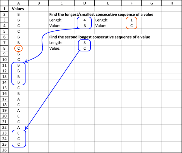
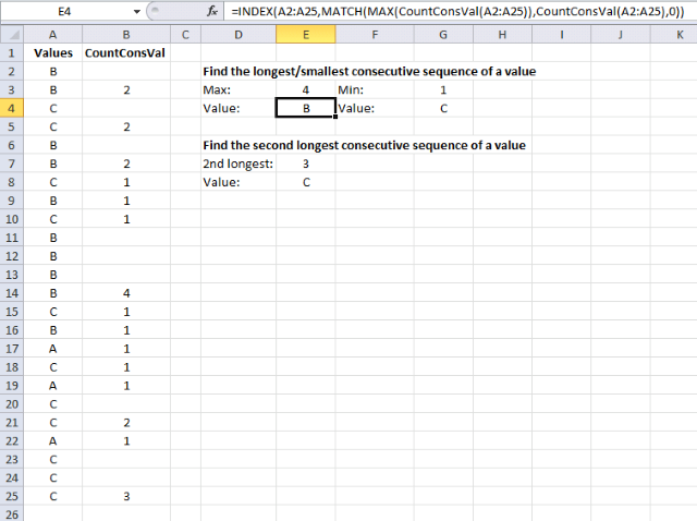
The array formula in cell D3 returns the the length of longest consecutive sequence of a value in column A. Cell D4 returns the value of the longest consecutive sequence in column A.
Cell F3 returns the length of the shortest consecutive sequence of a value in column A and cell F4 returns the value of the smallest consecutive sequence in column A.
5.1. Length of the most repeated grouped value
The array formula in cell D3 calculates how many cells contain the same given value repeated. It returns four in cell D3 because value "B" is repeated four times and is adjacent to each other in cell range A11:A14.
Array formula in cell D3:
How to enter an array formula
- Select cell
- Copy/Paste the formula to the formula bar
- Press and hold CTRL + SHIFT simultaneously
- Press Enter once
- Release all keys
Update 3-18-2021, Excel 365 formula:
Explaining formula in cell D3
Step 1 - Compare values in cell ranges
The less than and the greater than characters combined checks if a value is not equal to another value, it returns TRUE if not equal and FALSE if equal.
The second cell range is offset by 1, this makes the comparison check the following value which makes it easy to calculate the number of repeated values in a column.
$A$2:$A$25<>$A$3:$A$26
becomes
({"B"; "B"; "C"; "C"; "B"; "B"; "C"; "B"; "C"; "B"; "B"; "B"; "B"; "C"; "B"; "A"; "C"; "A"; "C"; "C"; "A"; "C"; "C"; "C"}<>{"B"; "C"; "C"; "B"; "B"; "C"; "B"; "C"; "B"; "B"; "B"; "B"; "C"; "B"; "A"; "C"; "A"; "C"; "C"; "A"; "C"; "C"; "C"; 0}
and returns
{FALSE; TRUE; FALSE; TRUE; FALSE; TRUE; TRUE; TRUE; TRUE; FALSE; FALSE; FALSE; TRUE; TRUE; TRUE; TRUE; TRUE; TRUE; FALSE; TRUE; TRUE; FALSE; FALSE; TRUE}
Step 2 - Replace TRUE with corresponding row number
The IF function returns one value if the logical test is TRUE and another value if the logical test is FALSE.
IF($A$2:$A$25<>$A$3:$A$26, "", MATCH(ROW($A$2:$A$25), ROW($A$2:$A$25)))
becomes
IF({FALSE; TRUE; FALSE; TRUE; FALSE; TRUE; TRUE; TRUE; TRUE; FALSE; FALSE; FALSE; TRUE; TRUE; TRUE; TRUE; TRUE; TRUE; FALSE; TRUE; TRUE; FALSE; FALSE; TRUE}, "", MATCH(ROW($A$2:$A$25), ROW($A$2:$A$25)))
becomes
IF({FALSE; TRUE; FALSE; TRUE; FALSE; TRUE; TRUE; TRUE; TRUE; FALSE; FALSE; FALSE; TRUE; TRUE; TRUE; TRUE; TRUE; TRUE; FALSE; TRUE; TRUE; FALSE; FALSE; TRUE}, "", {1; 2; 3; 4; 5; 6; 7; 8; 9; 10; 11; 12; 13; 14; 15; 16; 17; 18; 19; 20; 21; 22; 23; 24})
and returns
{1; ""; 3; ""; 5; ""; ""; ""; ""; 10; 11; 12; ""; ""; ""; ""; ""; ""; 19; ""; ""; 22; 23; ""}
Step 3 - Calculate frequency
The FREQUENCY function calculates how often values occur within a range of values and returns a vertical array of numbers. It returns an array that is one more item larger than the bins_array.
FREQUENCY(IF($A$2:$A$25<>$A$3:$A$26, "", MATCH(ROW($A$2:$A$25), ROW($A$2:$A$25))), IF($A$2:$A$25<>$A$3:$A$25, MATCH(ROW($A$2:$A$25), ROW($A$2:$A$25)) , ""))
becomes
FREQUENCY({1; ""; 3; ""; 5; ""; ""; ""; ""; 10; 11; 12; ""; ""; ""; ""; ""; ""; 19; ""; ""; 22; 23; ""}, {""; 2; ""; 4; ""; 6; 7; 8; 9; ""; ""; ""; 13; 14; 15; 16; 17; 18; ""; 20; 21; ""; ""; 24})
and returns
{1; 1; 1; 0; 0; 0; 3; 0; 0; 0; 0; 0; 1; 0; 2; 0}
Step 4 - Calculate max number in the array
The MAX function returns the largest number in a cell range or array.
MAX(FREQUENCY(IF($A$2:$A$25<>$A$3:$A$26, "", MATCH(ROW($A$2:$A$25), ROW($A$2:$A$25))), IF($A$2:$A$25<>$A$3:$A$25, MATCH(ROW($A$2:$A$25), ROW($A$2:$A$25)) ,""))+1)
becomes
MAX({1; 1; 1; 0; 0; 0; 3; 0; 0; 0; 0; 0; 1; 0; 2; 0}+1)
becomes
MAX({2; 2; 2; 1; 1; 1; 4; 1; 1; 1; 1; 1; 2; 1; 3; 1})
and returns 4.
5.2. Extract most repeated grouped value
The image above demonstrates a formula in cell D4 that extracts the most repeated adjacent value in column A.
Array formula in cell D4:
Update 3-18-2021, Excel 365 formula in cell D4:
Explaining formula in cell D4
Step 1 - Compare cell ranges and return corresponding row number if TRUE
The IF function returns one value if the logical test is TRUE and another value if the logical test is FALSE.
IF($A$2:$A$25<>$A$3:$A$26, MATCH(ROW($A$2:$A$25), ROW($A$2:$A$25)), "")
becomes
IF({FALSE; TRUE; FALSE; TRUE; FALSE; TRUE; TRUE; TRUE; TRUE; FALSE; FALSE; FALSE; TRUE; TRUE; TRUE; TRUE; TRUE; TRUE; FALSE; TRUE; TRUE; FALSE; FALSE; TRUE}, MATCH(ROW($A$2:$A$25), ROW($A$2:$A$25)), "")
becomes
IF({FALSE; TRUE; FALSE; TRUE; FALSE; TRUE; TRUE; TRUE; TRUE; FALSE; FALSE; FALSE; TRUE; TRUE; TRUE; TRUE; TRUE; TRUE; FALSE; TRUE; TRUE; FALSE; FALSE; TRUE}, {1; 2; 3; 4; 5; 6; 7; 8; 9; 10; 11; 12; 13; 14; 15; 16; 17; 18; 19; 20; 21; 22; 23; 24}, "")
and returns
{""; 2; ""; 4; ""; 6; 7; 8; 9; ""; ""; ""; 13; 14; 15; 16; 17; 18; ""; 20; 21; ""; ""; 24}
Step 2 - Compare cell ranges and return corresponding row number if FALSE
IF($A$2:$A$25<>$A$3:$A$26, "", MATCH(ROW($A$2:$A$25), ROW($A$2:$A$25)))
becomes
IF({FALSE; TRUE; FALSE; TRUE; FALSE; TRUE; TRUE; TRUE; TRUE; FALSE; FALSE; FALSE; TRUE; TRUE; TRUE; TRUE; TRUE; TRUE; FALSE; TRUE; TRUE; FALSE; FALSE; TRUE}, "", MATCH(ROW($A$2:$A$25), ROW($A$2:$A$25)))
becomes
IF({FALSE; TRUE; FALSE; TRUE; FALSE; TRUE; TRUE; TRUE; TRUE; FALSE; FALSE; FALSE; TRUE; TRUE; TRUE; TRUE; TRUE; TRUE; FALSE; TRUE; TRUE; FALSE; FALSE; TRUE}, "", {1; 2; 3; 4; 5; 6; 7; 8; 9; 10; 11; 12; 13; 14; 15; 16; 17; 18; 19; 20; 21; 22; 23; 24})
and returns
{1; ""; 3; ""; 5; ""; ""; ""; ""; 10; 11; 12; ""; ""; ""; ""; ""; ""; 19; ""; ""; 22; 23; ""}
Step 4 - Calculate the frequency of repeated values in column A
The FREQUENCY function calculates how often values occur within a range of values and returns a vertical array of numbers. It returns an array that is one more item larger than the bins_array.
FREQUENCY(IF($A$2:$A$25<>$A$3:$A$26, "", MATCH(ROW($A$2:$A$25), ROW($A$2:$A$25))), IF($A$2:$A$25<>$A$3:$A$26, MATCH(ROW($A$2:$A$25), ROW($A$2:$A$25)), ""))+1
becomes
FREQUENCY({1; ""; 3; ""; 5; ""; ""; ""; ""; 10; 11; 12; ""; ""; ""; ""; ""; ""; 19; ""; ""; 22; 23; ""}, {""; 2; ""; 4; ""; 6; 7; 8; 9; ""; ""; ""; 13; 14; 15; 16; 17; 18; ""; 20; 21; ""; ""; 24})+1
becomes
{1; 1; 1; 0; 0; 0; 3; 0; 0; 0; 0; 0; 1; 0; 2; 0} + 1
and returns
{2; 2; 2; 1; 1; 1; 4; 1; 1; 1; 1; 1; 2; 1; 3; 1}
Step 5 - Calculate largest value in array
The MAX function returns the largest number in a cell range or array.
MAX(FREQUENCY(y, x)+1)
becomes
MAX({2; 2; 2; 1; 1; 1; 4; 1; 1; 1; 1; 1; 2; 1; 3; 1})
and returns 4.
Step 6 - Find the position in array
The MATCH function returns a number representing the relative position af a given value in a cell range or array.
MATCH(MAX(FREQUENCY(IF($A$2:$A$25<>$A$3:$A$26, MATCH(ROW($A$2:$A$25), ROW($A$2:$A$25)),""), IF($A$2:$A$25<>$A$3:$A$26, MATCH(ROW($A$2:$A$25), ROW($A$2:$A$25)), ""))+1), FREQUENCY(IF($A$2:$A$25<>$A$3:$A$26, MATCH(ROW($A$2:$A$25), ROW($A$2:$A$25)),""), IF($A$2:$A$25<>$A$3:$A$26, MATCH(ROW($A$2:$A$25), ROW($A$2:$A$25)), ""))+1, 0)
becomes
MATCH(4, {2; 2; 2; 1; 1; 1; 4; 1; 1; 1; 1; 1; 2; 1; 3; 1}, 0)
and returns 7.
Step 7 - Calculate k-th smallest value
The SMALL function returns the k-th smallest number from a cell range or array.
SMALL(IF($A$2:$A$25<>$A$3:$A$26, MATCH(ROW($A$2:$A$25), ROW($A$2:$A$25)), ""), MATCH(MAX(FREQUENCY(IF($A$2:$A$25<>$A$3:$A$26, MATCH(ROW($A$2:$A$25), ROW($A$2:$A$25)),""), IF($A$2:$A$25<>$A$3:$A$26, MATCH(ROW($A$2:$A$25), ROW($A$2:$A$25)), ""))+1), FREQUENCY(IF($A$2:$A$25<>$A$3:$A$26, MATCH(ROW($A$2:$A$25), ROW($A$2:$A$25)),""), IF($A$2:$A$25<>$A$3:$A$26, MATCH(ROW($A$2:$A$25), ROW($A$2:$A$25)), ""))+1, 0))
becomes
SMALL({""; 2; ""; 4; ""; 6; 7; 8; 9; ""; ""; ""; 13; 14; 15; 16; 17; 18; ""; 20; 21; ""; ""; 24}, 7)
and returns 13.
Step 8 - Return value
The INDEX function returns a value from a given cell range or array based on a row and column number.
INDEX($A$2:$A$25, SMALL(IF($A$2:$A$25<>$A$3:$A$26, MATCH(ROW($A$2:$A$25), ROW($A$2:$A$25)), ""), MATCH(MAX(FREQUENCY(IF($A$2:$A$25<>$A$3:$A$26, "", MATCH(ROW($A$2:$A$25), ROW($A$2:$A$25))), IF($A$2:$A$25<>$A$3:$A$26, MATCH(ROW($A$2:$A$25), ROW($A$2:$A$25)), ""))+1), FREQUENCY(IF($A$2:$A$25<>$A$3:$A$26, "", MATCH(ROW($A$2:$A$25), ROW($A$2:$A$25))), IF($A$2:$A$25<>$A$3:$A$26, MATCH(ROW($A$2:$A$25), ROW($A$2:$A$25)), ""))+1, 0)))
becomes
INDEX($A$2:$A$25, 13)
and returns "B" in cell D4.
5.3. Length of the shortest consecutive sequence of a value
Array formula in cell F3:
5.4. Value of the shortest consecutive sequence
Array formula in cell F4:
5.5. Length of second longest consecutive sequence of a value
Array formula in cell D7:
5.6. Value of the second-longest consecutive sequence
Array formula in cell D8:
If you are interested in learning and constructing array formulas, check out my Advanced excel course.
6. Count groups of repeated values per row
I have a worksheet that has rows, each containing sequential groupings of values of "1" and "0". These alternate across 1800 columns of data.
My question: how do I count the number of groupings of each? In other words, across those 1800 columns, how many arrays of value 1 and how many arrays of value 0 do I have?
Thanks.
Joe
Answer:
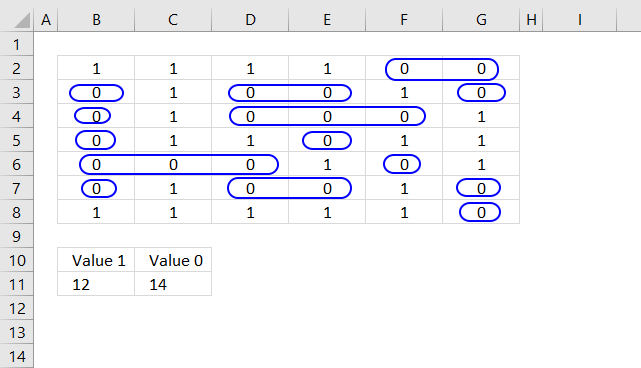
I am using a much smaller size to more easily show how the formulas work and what the functions used return.
There are 14 groups of value 0 (zero) per row in cell range B2:G8 and 12 groups of value 1. The image above shows 14 blue circles around each group of value 0 to demonstrate how the formula below works.
Regular formula in cell B11:
Array formula in cell C11:
This formula is different because Excel evaluates a blank cell as 0 (zero), this makes it impossible to use the same formula as in cell B11.
How to create an array formula
- Copy formula above.
- Select cell C11 with mouse.
- Paste formula (keyboard shortcut CTRL + v)
- Press and hold CTRL + SHIFT simultaneously.
- Press Enter once
- Release all keys.
Explaining array formula in cell C11
The formula in cell C11 is slightly more complicated than the formula in cell B11, they are however so similar that I will only explain the formula in cell C11.
Step 1 - Check if cell is blank
The ISBLANK function returns TRUE if the cell is blank and FALSE if not blank, no surprises here.
ISBLANK(A2:F8)
becomes
ISBLANK({0, 1, 1, 1, 1, 0; 0, 0, 1, 0, 0, 1; 0, 0, 1, 0, 0, 0; 0, 0, 1, 1, 0, 1; 0, 0, 0, 0, 1, 0; 0, 0, 1, 0, 0, 1; 0, 1, 1, 1, 1, 1})
and returns
{TRUE, FALSE, FALSE, FALSE, FALSE, FALSE; TRUE, FALSE, FALSE, FALSE, FALSE, FALSE; TRUE, FALSE, FALSE, FALSE, FALSE, FALSE; TRUE, FALSE, FALSE, FALSE, FALSE, FALSE; TRUE, FALSE, FALSE, FALSE, FALSE, FALSE; TRUE, FALSE, FALSE, FALSE, FALSE, FALSE; TRUE, FALSE, FALSE, FALSE, FALSE, FALSE}.
Step 2 - If blank return a blank
The IF function returns a blank if the logical expression ISBLANK(A2:F8) returns TRUE and returns the number itself if FALSE.
IF(ISBLANK(A2:F8),"",A2:F8)
becomes
IF({TRUE, FALSE, FALSE, FALSE, FALSE, FALSE; TRUE, FALSE, FALSE, FALSE, FALSE, FALSE; TRUE, FALSE, FALSE, FALSE, FALSE, FALSE; TRUE, FALSE, FALSE, FALSE, FALSE, FALSE; TRUE, FALSE, FALSE, FALSE, FALSE, FALSE; TRUE, FALSE, FALSE, FALSE, FALSE, FALSE; TRUE, FALSE, FALSE, FALSE, FALSE, FALSE},"",A2:F8)
becomes
IF({TRUE, FALSE, FALSE, FALSE, FALSE, FALSE; TRUE, FALSE, FALSE, FALSE, FALSE, FALSE; TRUE, FALSE, FALSE, FALSE, FALSE, FALSE; TRUE, FALSE, FALSE, FALSE, FALSE, FALSE; TRUE, FALSE, FALSE, FALSE, FALSE, FALSE; TRUE, FALSE, FALSE, FALSE, FALSE, FALSE; TRUE, FALSE, FALSE, FALSE, FALSE, FALSE}, "", {0, 1, 1, 1, 1, 0; 0, 0, 1, 0, 0, 1; 0, 0, 1, 0, 0, 0; 0, 0, 1, 1, 0, 1; 0, 0, 0, 0, 1, 0; 0, 0, 1, 0, 0, 1; 0, 1, 1, 1, 1, 1})
and returns
{"",1,1,1,1,0;"",0,1,0,0,1;"",0,1,0,0,0;"",0,1,1,0,1;"",0,0,0,1,0;"",0,1,0,0,1;"",1,1,1,1,1}
These two steps are necessary due to Excel not being able to compare a 0 (zero) with an empty cell. Excel evaluates an empty cell as 0 (zero).
Step 3 - Compare arrays
This step compares values in order to identify groups of repeated values.
(B2:G8<>IF(ISBLANK(A2:F8),"",A2:F8))
becomes
(B2:G8<>{"",1,1,1,1,0;"",0,1,0,0,1;"",0,1,0,0,0;"",0,1,1,0,1;"",0,0,0,1,0;"",0,1,0,0,1;"",1,1,1,1,1})
becomes
({0, 1, 1, 1, 1, 0; 0, 0, 1, 0, 0, 1; 0, 0, 1, 0, 0, 0; 0, 0, 1, 1, 0, 1; 0, 0, 0, 0, 1, 0; 0, 0, 1, 0, 0, 1; 0, 1, 1, 1, 1, 1}<>{"",1,1,1,1,0;"",0,1,0,0,1;"",0,1,0,0,0;"",0,1,1,0,1;"",0,0,0,1,0;"",0,1,0,0,1;"",1,1,1,1,1})
and returns
{TRUE, FALSE, FALSE, FALSE, TRUE, FALSE; TRUE, TRUE, TRUE, FALSE, TRUE, TRUE; TRUE, TRUE, TRUE, FALSE, FALSE, TRUE; TRUE, TRUE, FALSE, TRUE, TRUE, FALSE; TRUE, FALSE, FALSE, TRUE, TRUE, TRUE; TRUE, TRUE, TRUE, FALSE, TRUE, TRUE; TRUE, FALSE, FALSE, FALSE, FALSE, TRUE}
Step 4 - Check if cell is 0 (zero)
This step filters groups of zeros, we don't want to count 1's.
B2:G8=0
becomes
{0, 1, 1, 1, 1, 0; 0, 0, 1, 0, 0, 1; 0, 0, 1, 0, 0, 0; 0, 0, 1, 1, 0, 1; 0, 0, 0, 0, 1, 0; 0, 0, 1, 0, 0, 1; 0, 1, 1, 1, 1, 1}=0
and returns
{FALSE, FALSE, FALSE, FALSE, TRUE, TRUE; TRUE, FALSE, TRUE, TRUE, FALSE, TRUE; TRUE, FALSE, TRUE, TRUE, TRUE, FALSE; TRUE, FALSE, FALSE, TRUE, FALSE, FALSE; TRUE, TRUE, TRUE, FALSE, TRUE, FALSE; TRUE, FALSE, TRUE, TRUE, FALSE, TRUE; FALSE, FALSE, FALSE, FALSE, FALSE, TRUE}
Step 5 - Multiply arrays
(B2:G8<>IF(ISBLANK(A2:F8),"",A2:F8))*(B2:G8=0)
becomes
{TRUE, FALSE, FALSE, FALSE, TRUE, FALSE; TRUE, TRUE, TRUE, FALSE, TRUE, TRUE; TRUE, TRUE, TRUE, FALSE, FALSE, TRUE; TRUE, TRUE, FALSE, TRUE, TRUE, FALSE; TRUE, FALSE, FALSE, TRUE, TRUE, TRUE; TRUE, TRUE, TRUE, FALSE, TRUE, TRUE; TRUE, FALSE, FALSE, FALSE, FALSE, TRUE}*{FALSE, FALSE, FALSE, FALSE, TRUE, TRUE; TRUE, FALSE, TRUE, TRUE, FALSE, TRUE; TRUE, FALSE, TRUE, TRUE, TRUE, FALSE; TRUE, FALSE, FALSE, TRUE, FALSE, FALSE; TRUE, TRUE, TRUE, FALSE, TRUE, FALSE; TRUE, FALSE, TRUE, TRUE, FALSE, TRUE; FALSE, FALSE, FALSE, FALSE, FALSE, TRUE}
and returns
{0, 0, 0, 0, 1, 0; 1, 0, 1, 0, 0, 1; 1, 0, 1, 0, 0, 0; 1, 0, 0, 1, 0, 0; 1, 0, 0, 0, 1, 0; 1, 0, 1, 0, 0, 1; 0, 0, 0, 0, 0, 1}.
Step 6 - Sum values
The SUM function adds the numbers in the array and returns a total.
SUM((B2:G8<>IF(ISBLANK(A2:F8),"",A2:F8))*(B2:G8=0))
becomes
SUM({0, 0, 0, 0, 1, 0; 1, 0, 1, 0, 0, 1; 1, 0, 1, 0, 0, 0; 1, 0, 0, 1, 0, 0; 1, 0, 0, 0, 1, 0; 1, 0, 1, 0, 0, 1; 0, 0, 0, 0, 0, 1})
and returns 14 in cell C11.
Sequence category
Excel has a great built-in tool for creating number series named Autofill. The tool is great, however, in some situations, […]
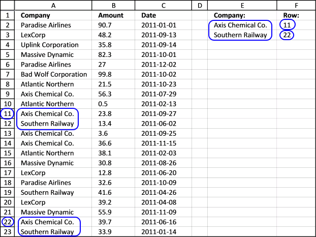
This article demonstrates array formulas that identify two search values in a row or in a sequence. The image above […]
Excel categories
38 Responses to “Repeat values across cells”
Leave a Reply
How to comment
How to add a formula to your comment
<code>Insert your formula here.</code>
Convert less than and larger than signs
Use html character entities instead of less than and larger than signs.
< becomes < and > becomes >
How to add VBA code to your comment
[vb 1="vbnet" language=","]
Put your VBA code here.
[/vb]
How to add a picture to your comment:
Upload picture to postimage.org or imgur
Paste image link to your comment.
Again want to thank you Oscar!
You saved me a lot of time and when I saw your formula – simple and clever, I want to have just a part from your knowledge in the field of array formulas and Excel!
I will modify a little bit a formula to preserve of #N/A and make it more flexible:
=IF(ROW()-ROW($A$6)<=SUM($B$1:$B$4)-1;INDEX($A$1:$A$4;MATCH(FALSE; COUNTIF($A$5:A5;$A$1:$A$4)=$B$1:$B$4;0));"")
Even without that the formula is perfect!
Best regards
Todor
P.S. I think that I asked you on the past, but can you recommend me some resources in connection with array formulas?
the countif formula doesn't return true or false in my spreadsheet even after I restarted Excel... :(
I need to generate result from the below table
Col A Col B Col C
Model Model Group Number of times
Oasis-LS1 oasis 0.5
Oasis-LS2 oasis 1
Oasis-LS3 oasis 0.5
Phara-1 phara 1.5
Phara-2 phara 2
to
Col A Col B
Model
Oasis Oasis-LS1 (0.5); Oasis-LS3 (0.5)
Oasis Oasis LS1
Phara-1 Phara-1
Phara-1 Phara-1 (0.5)
Phara-1 Phara-1
Phara-1 Phara-1
I tried using countif and it didn't return true or false.... Can you please help?
Well done. Clever formula.
//Ola
Hi Oscar,
Great Job.. Is this possible to repeat the range according to criteria in loop.. like below.
Z 5
Y 2
X 1
W 4
then Z 5 Times, Y 2 Times.... but in series
Z
Y
X
W
Z
Y
W
Z
W
Z
W
Z
Regards,
Deb
Debraj,
read this:
Repeat the range according to criteria in loop
Hi Oscar,
OOPS brillinat.. just impressed
Thanks for teaching : "there are lots of thing to check ISERROR ("A") .. Only " " is not the limit.. :)"
Regards,
Deb
Hello Oscar,
Thanks for wonderfull website.
I would like to draw attention with respect to "Repeat the range according to criteria in loop". If A1:B4 is having formulae instead of text, output have blank cell in between.
Regards,
S
Shailesh
I would like to draw attention with respect to "Repeat the range according to criteria in loop". If A1:B4 is having formulae instead of text, output have blank cell in between.
It works for me, please check your cell references. I am guessing they reference a blank cell.
super and extremely efficient formula...
Ola and chrisham,
thank you!
hi oscar
thanks again for your formula
how to change 1 value and keep other columns same
eg
col1 col2 col3
item1 a1 b1
item2
item3
item4
output
col1 col2 col3
item1 a1 b1
item2 a1 b1
item3 a1 b1
item4 a1 b1
dont want fill down bcoz lot of items with lots of a's and b's
any macro?
thanks
krishna
Krishna,
When you enter a value in column A, column B and C are automatically filled with values a1 and b1?
hi oscar ,
thanks for giving an option to upload the image.
this is what i wanted
https://postimg.org/image/vgtdw40wj/9b6c7581/
Krishna,
Get the Excel *.xlsm file
Repeat-values-vba.xlsm
[…] Repeat values […]
This reminded me of a article I wrote a while back, only I took the perspective of using this methodology to calculate win/loss streaks for a sports team. There's a lot of cool stuff you can do with this consecutive sequence formula!
https://www.thespreadsheetguru.com/blog/2014/6/29/formulas-to-calculate-longest-current-win-streaks?rq=streak
Chris Macro,
Yes, there is a lot of cool stuff you can do I only wish I could come up with shorter formulas.
The FREQUENCY function really saved me, I thought quite a while before figuring out how to solve this problem.
Thanks for sharing your post.
I got an email from David, his formulas are a lot smaller.
Formula in D4:
=INDEX($A$2:$A$25,AGGREGATE(14, 6, ROW($A$3:$A$26)-2/(FREQUENCY(IF($A$2:$A$25=$A$3:$A$26, ROW($A$2:$A$25)), ($A$2:$A$25<>$A$3:$A$26)*ROW($A$2:$A$25))=(D3-1)), 1), 0)
Get his workbook:
https://www.get-digital-help.com/wp-content/uploads/2014/11/longest-consecutive-sequence-1.xlsx
First off, you show your formula starting in cell B3... you need to adjust it so that it starts in cell B2, otherwise you will not show a 1 in cell B2 if cell A2 differs from cell A3.
Second, here is a much simpler, still array-entered, formula, placed in cell B2 and copied down, that appears to produce the same output as your formula...
=IF(A3<>A4,ROW()-MAX(IF(A$1:A2<>A3,ROW(A$1:A2))),"")
Sorry, I posted the wrong formula, plus it looks like the comment processor ate my less than greater than symbol. Here is the correct array-entered formula, rearrange to eliminate the display problem...
=IF(A2=A3,"",ROW()-MAX(IF(A$1:A1<>A2,ROW(A$1:A1))))
D@MN! I missed that the comment processor ate a second less than, greater than symbols in my formula. Here now is the correct [b]array-entered[/b] formula (rearranged so that there are no less than, greater than symbols at all)..
=IF(A2=A3,"",ROW()-MAX(IF(A$1:A1=A2,,ROW(A$1:A1))))
Rick Rothstein (MVP - Excel),
Your formulas work fine, thanks. So much better and smaller than mine.
I am sorry for wordpress eating your less/greater than signs, I try to edit your comments as soon as I can.
Hello oscar I tried your code for repeating value (repeat values.xlsx), i am uploading the file i am getting #value! error
How can i do this with colorformatted cells?. All the cells have the same value (1) the range is A1:A99999 and some rows are colorformatted with red using a different sheeth(table) and vba code.
I have this sequence of C2: O2,
2 1 2 X X X 2 X 1 X 2 X 2
I need you to return the largest consecutive sequence:
X should be 3
2 should be 2
1 should be 1
x and 2 should be 4.
Another example:
X 2 X 1 1 X 1 1 X 1 1 1 2
1 X must be
2 must be 1
1 must be 5
x and 2 should be 2.
Tenho esta sequencia de C2:O2,
2 X X X 1 2 2 X 1 2 X X 2
Preciso que retorne a maior sequencia consecutiva de:
X deve ser 3
2 deve ser 2
1 deve ser 1
x e 2 deve ser 4 .
Outro exemplo:
X 2 1 X 1 X 1 1 1 1 1 2 X
X deve ser 1
2 deve ser 1
1 deve ser 5
x e 2 deve ser 2 .
Please helpme, If I change the numnber 1 by zero.
1. How many consecutive zero 2nd logest?
2. How many consecutive zero from left to rỉght in a row?
Thanks
Okido
The values in column B show how many consecutive values there are in column A, for each group.
I am a newbie at this. I have been trying to follow your instruction on how to do it but I can not seem to do it right. Copy-pasting the udf down the rows does not seem to work for me. Instead of alphabets in column A, I used their corresponding ordinal numbers, such A = 1, B = 2, C = 3. For column B, instead of just the number, it must include the letter it counted, like "3 C's" in B25 cell which is "3" only. I hope you could help me with this. Thank you.
liam,
Copy-pasting the udf down the rows does not seem to work for me.
No, the following steps allows you to enter the UDF as an array formula.
1. Select cell range B2:B25.
2. Type: =CountConsVal(A2:A25)&" "&CHAR(A2:A25+64)&"'S "
3. Press and hold CTRL + SHIFT simultaneously.
4. Press Enter once.
5. Release all keys
Instead of alphabets in column A, I used their corresponding ordinal numbers, such A = 1, B = 2, C = 3. For column B, instead of just the number, it must include the letter it counted, like "3 C's" in B25 cell which is "3" only.
See formula in step 2 above.
Thank you so much for the help. It worked perfectly!
Hi,
The formula does not work when the data is displayed horizontally.
Hi. I am trying to generate a chart that show how many time each number in the array followed the others.
My array is 6 columns by 2600 rows is a random list the first column the numbers go from 1 to 48, second 2-49; 3-50; 4-51; 5-52; 6-53.
thank you for reading this post.
Jeyner Lopez,
Can you explain "how many time each number in the array followed the others." in greater detail?
Hi,
I am trying to find the longest consecutive sequence of different words in a column before one of the words is repeated, then display a list of those words. Hoping someone could please assist with an Excel formula for this. Thank-you.
Thank you for all your information, I appreciate it. If I'm copying the formula of D3 into Google Sheets, it's not working. It gives the number 2, while using the same values in column A as you. The formula of D4 turns in the right value (B). Do you know if the formula needs some change to work in google?
do u have version for google sheets
Thanks for this. It works. However, what do I do if I have blank cells in my array, that I do not wish to be counted?
To use your example: Imagine cells A11:A14 did not contain "B" in them, but rather were left blank. Then your formula would still say the longest consecutive sequence is 4, with a value "" (blank).
Obviously that is not a desired outcome. In this case the longest consecutive sequence would be A23:A25. A sequence of 3 Cs.
Can you please suggest a solution?
Thank you in advance!
Kind regards,
Deyan