How to do tiered calculations in one formula
The image above demonstrates a formula that calculates tiered values based on a tier table and returns a total. This kind of formula is often used to calculate
- Commissions. Money earned for selling something.
- Bonuses. Extra money for good work.
- Pricing. The cost.
- Fees or charges. Extra costs for services.
- Discounts. A price cut or lower cost.
- Volume pricing. Lower prices for buying more.
- Volume rebate. Money back for buying a lot.
- Taxations. Money paid to the government.
- Performance incentives. Rewards for working well.
I have written an article about how to Use price ranges to determine discounts, it also explains how to calculate linear discounts.
What is a tier calculation or progressive calculation?
In a tiered calculation, different portions of a total value are calculated at different rates based on predefined thresholds and percentages. Each tier has its own percentage rate. Only the amount within each tier is calculated at that tier's rate.
Imagine a commission structure with these tiers:
- 4.5% for sales up to $100,000
- 2% for sales between $100,000 and $250,000
- 1.2% for sales between $ 250,000 and $500,000
- .2% for sales between $ 500,000 and $999,999
For a total sale of $150,000, the calculation would break down like this:
- First $100,000: $100,000 × 4.5% = $4,500
- Next $50,000: (from $100,000 to $150,000): $50,000 × 2% = $1,000
Total commission: $4,500 + $1,000 = $5,500
The table in the image above shows the different thresholds or levels that a specific percentage applies to, if an amount is larger than the first level then multiple calculations are necessary in order to calculate the total. The formula takes care of these additional calculations as well, no need for helper columns.
Table of contents
1. How to do tiered calculations in one formula
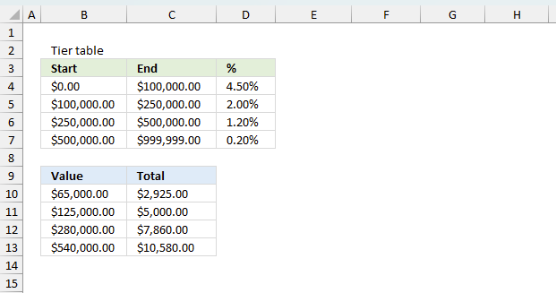
The image above shows the tier table in cells B3:D7 it contains a start value and an end value in columns B and C respectively. Column D contains the percentage for that range. For example a value between 0 (zero) and 100,000 has a percentage of 4.5
Cells B10:B13 contains these values: 65,000 125,000 280,000 and 540,000
Formula in cell C10:
There are four different values B10:B13 in order to demonstrate how the total changes based on the percentage and levels used, I will explain below how each value is calculated. The first value 65,000 is explained below.
1.1 Explaining calculations
1.1.1 Example 1 - $65,000
The formula in cell C10 returns 2,925 based on $65 000, here is how that number is calculated: 65,000 * 4.5% = 2,925
The amount is in cell B10 and the calculation is in cell C10, see the image above.
| Amount | Percentage | Result |
| 65,000 | 4.5% | 2,925 |
| Total | 2,925 |
The formula returns 2,950.00 in cell C10 which matches the total in the table above.
1.1.2 Example 2 - $125,000
$125,000 returns $5,000. 100,000 * 4.5% = 4,500. 25,000 * 2% = 500. 4,500 + 500 = 5,000.
The amount is in cell B11 and the calculation is in cell C11, see the image above.
| Amount | Percentage | Result |
| 100 000 | 4.5% | 4 500 |
| 25 000 | 2% | 500 |
| Total | 5 000 |
The formula returns 5,000.00 in cell C11 which matches the total in the table above.
1.1.3 Example 3 - $280 000
$280,000 returns $7,860. 100,000 * 4.5% = 4,500. 150,000 * 2% = 3,000. 30,000 * 1.2% = 360. 4,500 + 3,000 + 360 = 7,860
The amount is in cell B12 and the calculation is in cell C12, see the image above.
| Amount | Percentage | Result |
| 100 000 | 4.5% | 4 500 |
| 150 000 | 2% | 3 000 |
| 30 000 | 1.2% | 360 |
| Total | 7 860 |
The formula returns 7,860.00 in cell C12 which matches the total in the table above.
1.1.4 Example 4 - $540,000
$540,000 returns $10,580. 100,000 * 4.5% = 4,500. 150,000 * 2% = 3,000. 250,000 * 1.2% = 3,000. 40,000 * 0.2% = 80. 4,500 + 3,000 + 3,000 + 80 = 10,580.
The amount is in cell B13 and the calculation is in cell C13, see the image above.
| Amount | Percentage | Result |
| 100,000 | 4.5% | 4,500 |
| 150,000 | 2% | 3,000 |
| 250,000 | 1.2% | 3,000 |
| 40,000 | 0.2% | 80 |
| Total | 10,580 |
The formula returns 10,580.00 in cell C12 which matches the total in the table above.
1.2 Explaining formula in cell C10
The formula contains two SUMPRODUCT functions, the first one calculates the result based on the amount that is above a specific level and the corresponding percentage.
The second SUMPRODUCT function calculates tiered values based on the amounts up to the reached level and their corresponding percentages. The formula then adds those numbers and returns the total.
Recommended article: How to return a value if lookup value is in a range
Step 1 - First SUMPRODUCT function
The first two logical expressions determine which tier the amount in cell B10 reaches.
(B10<=$C$4:$C$7)* (B10>$B$4:$B$7)
becomes
(65000<={100000; 250000; 500000; 999999})*(65000>{0; 100000; 250000; 500000})
becomes
({TRUE; TRUE; TRUE; TRUE})*({TRUE; FALSE; FALSE; FALSE})
and returns {1; 0; 0; 0}.
Step 2 - Subtract value with tier levels
The parentheses let you control the order of operation, we want to subtract before we multiply the arrays in order to get the correct result we are looking for.
(B10- $B$4:$B$7)
becomes
(65000 - {0; 100000; 250000; 500000})
and returns {65000; -35000; -185000; -435000}.
Step 3 - Multiply arrays
(B10<$C$4:$C$7)*(B10>$B$4:$B$7)*(B10- $B$4:$B$7)* $D$4:$D$7
becomes
{1; 0; 0; 0}*{65000; -35000; -185000; -435000}*{0.045;0.02;0.012;0.002}
and returns {2925; 0; 0; 0}.
Step 4 - Add values
The SUMPRODUCT function calculates the product of corresponding values and then returns the sum of each multiplication.
SUMPRODUCT((B10<$C$4:$C$7)* (B10>$B$4:$B$7)* (B10- $B$4:$B$7)* $D$4:$D$7)
becomes
SUMPRODUCT({2925;0;0;0})
and returns 2925.
Step 5 - Second SUMPRODUCT function
((B10>$C$4:$C$7)* ($C$4:$C$7- $B$4:$B$7))* $D$4:$D$7
becomes
(65000>{100000;250000;500000;999999})*({100000;150000;250000;499999})*{0.045;0.02;0.012;0.002}
and returns {0;0;0;0}.
Step 6 - Add values in array
SUMPRODUCT(((B10>$C$4:$C$7)* ($C$4:$C$7- $B$4:$B$7))* $D$4:$D$7)
becomes
SUMPRODUCT({0;0;0;0})
and returns 0.
Step 7 - Add numbers
SUMPRODUCT((B10<=$C$4:$C$7)* (B10>$B$4:$B$7)* (B10- $B$4:$B$7)* $D$4:$D$7)+ SUMPRODUCT(((B10>$C$4:$C$7)* ($C$4:$C$7- $B$4:$B$7))* $D$4:$D$7)
becomes
2925 + 0
and returns 2925 in cell C10.
1.3 Final thoughts
The formula can be simplified to:
but that formula is harder for me to explain.
Excel 365 users can use this smaller dynamic array formula:
I recommend reading how to use VLOOKUP to calculate discounts, commissions, tariffs, charges, shipping costs, packaging expenses, or bonuses
2. How to do tiered calculations in one formula based on a condition

This example demonstrates a formula that uses multiple tier tables to calculate a total, a condition determines which table to use. The tier tables are merged to a larger table displayed in cell range B3:E15, they each have a designated shown color in column B. This color determines which table to use.
Formula in cell D18:
For example, cell B18 contains "Red" which determines which tier table to use. The value is in cell C18 which is 95,000 and the calculation is in cell D18 which displays 6,365. Here is how it is calculated: Tier table "Red" has a threshold of 0 - 100,000 and a rate of 6.7%. Value 95,000 is within the first threshold or limit. 0.067 * 95,000 = 6,365
Cell B19 contains "Blue" and the value in cell C19 is 125,000 and the total is 5,000 displayed in cell D19. Here is how it is calculated:
Tier table "Blue" has a threshold of
- 0 - 100,000 and a rate of 4.5%.
- 100,000 - 250,000, rate = 2%
Value 125,000 is within the second threshold or limit.
- First tier: 0.045 * 100,000 = 4,500
- Second tier: 0.02 * 25,000 = 500
The total is 4,500 + 500 = 5,000
The following formula works only in Excel 365, however, it does the same thing as the formula above but is much shorter and easier to adjust if your tier tables are larger or smaller.
Excel 365 dynamic array formula in cell D18:
3. Calculate total by tier and grand total
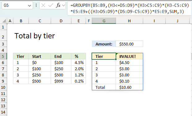
This example shows how to calculate the total by tier. The tier table is in cell range B6:E9, the amount is in cell H3. The differences between this formula and the formula described in section 1 are:
- This formula works only in Excel 365, it contains the new GROUPBY function which is only available in Excel 365.
- The formula in section 1 calculates a grand total, while this formula calculates the total for each tier and then calculates the grand total at the bottom.
Excel 365 dynamic array formula in cell G5:
The formula returns an array that spills to adjacent cells to the right and to cells below as far as needed. The array contains the tier number and the total for each tier based on the specified amount in cell H3. The last row in the array contains the grand total.
Tier 1 : 100 * 0.045 = 4.5
Tier 2 : 150 * 0.02 = 3
Tier 3 : 250 * 0.012 = 3
Tier 4 : 50 * 0.002 = 0.1
Total: 4.5 + 3 + 3 + 0.1 = 10.6
The top right container in the array contains a #VALUE! error which you can remove by using the IFERROR function, like this: =IFERROR(GROUPBY(....),"") Note that this replaces all errors with a blank which makes the formula harder to troubleshoot.
The formula in cell G5 is similar to the formula in section 1, read section 1 to understand how the formula works in greater detail.
4. Tiered calculations with multiple amounts
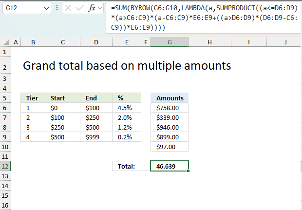
This example demonstrates how to calculate a grand total based on multiple amounts. The tier table is in cells B5:E9 and the amounts are in cells G6:G10. The following formula works only in Excel 365, it uses both the BYROW and LAMBDA functions which are only available in Excel 365.
Excel 365 dynamic formula in cell G12:
The formula in cell G12 returns 46.639, here is how that grand total is calculated:
Amount $758 has a total of $11.016, here is the calculation in detail:
Tier 1 : 100 * 0.045 = 4.5
Tier 2 : 150 * 0.02 = 3
Tier 3 : 250 * 0.012 = 3
Tier 4 : 258 * 0.002 = 0.516
Total: 4.5 + 3 + 3 + 0.516 = 11.016
Amount $339 has a total of $8.568, here is the calculation in detail:
Tier 1 : 100 * 0.045 = 4.5
Tier 2 : 150 * 0.02 = 3
Tier 3 : 89 * 0.012 = 1.068
Tier 4 : 0 * 0.002 = 0
Total: 4.5 + 3 + 1.068 + 0= 8.568
Amount $946 has a total of $11.392, here is the calculation in detail:
Tier 1 : 100 * 0.045 = 4.5
Tier 2 : 150 * 0.02 = 3
Tier 3 : 250 * 0.012 = 3
Tier 4 : 446 * 0.002 = 0.892
Total: 4.5 + 3 + 3 + 0.892 = 11.392
Amount $899 has a total of $11.298, here is the calculation in detail:
Tier 1 : 100 * 0.045 = 4.5
Tier 2 : 150 * 0.02 = 3
Tier 3 : 250 * 0.012 = 3
Tier 4 : 399 * 0.002 = 0.798
Total: 4.5 + 3 + 3 + 0.1 = 11.298
Amount $97 has a total of $11.016, here is the calculation in detail:
Tier 1 : 97 * 0.045 = 4.365
Tier 2 : 0 * 0.02 = 0
Tier 3 : 0 * 0.012 = 0
Tier 4 : 0 * 0.002 = 0
Total: 4.365 + 0 + 0 + 0 = 4.365
The grand total is 11.016 + 8.568 + 11.392 + 11.298 + 4.365 equals 46.639 which corresponds to the value in cell G12.
5. Total and grand total by amount
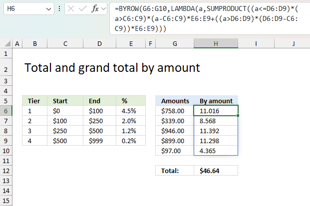
Section 4 described a formula that calculates the grand total of tier calculations based on multiple amounts. This example shows how to calculate totals by each amount in one array. The tier table is in cell B5:E9, the amounts are in cells G6:G10.
Excel 365 dynamic array formula in cell H6:
Amount $758 has a total of $11.016, here is the calculation in detail:
Tier 1 : 100 * 0.045 = 4.5
Tier 2 : 150 * 0.02 = 3
Tier 3 : 250 * 0.012 = 3
Tier 4 : 258 * 0.002 = 0.516
Total: 4.5 + 3 + 3 + 0.516 = 11.016
Amount $339 has a total of $8.568, here is the calculation in detail:
Tier 1 : 100 * 0.045 = 4.5
Tier 2 : 150 * 0.02 = 3
Tier 3 : 89 * 0.012 = 1.068
Tier 4 : 0 * 0.002 = 0
Total: 4.5 + 3 + 1.068 + 0= 8.568
Amount $946 has a total of $11.392, here is the calculation in detail:
Tier 1 : 100 * 0.045 = 4.5
Tier 2 : 150 * 0.02 = 3
Tier 3 : 250 * 0.012 = 3
Tier 4 : 446 * 0.002 = 0.892
Total: 4.5 + 3 + 3 + 0.892 = 11.392
Amount $899 has a total of $11.298, here is the calculation in detail:
Tier 1 : 100 * 0.045 = 4.5
Tier 2 : 150 * 0.02 = 3
Tier 3 : 250 * 0.012 = 3
Tier 4 : 399 * 0.002 = 0.798
Total: 4.5 + 3 + 3 + 0.1 = 11.298
Amount $97 has a total of $11.016, here is the calculation in detail:
Tier 1 : 97 * 0.045 = 4.365
Tier 2 : 0 * 0.02 = 0
Tier 3 : 0 * 0.012 = 0
Tier 4 : 0 * 0.002 = 0
Total: 4.365 + 0 + 0 + 0 = 4.365
The grand total is 11.016 + 8.568 + 11.392 + 11.298 + 4.365 equals 46.639 which corresponds to the value in cell H12.
6. Excel file
Find numbers in sum category
Table of Contents Identify numbers in sum using Excel solver Find numbers in sum - UDF Find positive and […]
Excelxor is such a great website for inspiration, I am really impressed by this post Which numbers add up to […]
Sum category
Andrew asks: LOVE this example, my issue/need is, I need to add the results. So instead of States and Names, […]
This article explains why your formula is not working properly, there are usually four different things that can go wrong. […]
Excel categories
30 Responses to “How to do tiered calculations in one formula”
Leave a Reply
How to comment
How to add a formula to your comment
<code>Insert your formula here.</code>
Convert less than and larger than signs
Use html character entities instead of less than and larger than signs.
< becomes < and > becomes >
How to add VBA code to your comment
[vb 1="vbnet" language=","]
Put your VBA code here.
[/vb]
How to add a picture to your comment:
Upload picture to postimage.org or imgur
Paste image link to your comment.
Thanks. This was super helpful.
What if my value in B10 is 100000. I am getting result as 0
Indresh,
You found an error in my formula. I have updated the formula and the uploaded file.
Thank you.
Why is it necessary to add the second sumproduct formula if you are reaching the same number with just the first formula?
THANKS, This is quite useful.
By any chance do you have banded interest rate excel
Say band 1 is from 0-5000 interest rate is 6% and Band 2 is 5001 to 12,000, INTEREST RATE IS 10%
If my balance is 6000 then interest to be applied is 10%
if my balance is 2000 then interest to be applied is 6%
TIA
Indresh Misha
Check out this article: https://www.get-digital-help.com/return-value-if-in-range-in-excel/
Brilliant, thanks a lot for all your help.
Oscar: You are a lifesaver. Thank you very much for this fantastic walkthrough!
You are welcome!
Hello,
What if I am looking to calculate partial payouts? Ex. rebates are earned in bands, but only for the amount in each band.
Say that we are looking to reward spending growth above a baseline.
The baseline is $100,000.
We create three achievement bands:
100% - 105%,
105% - 115%,
and greater than 115%.
Therefore all excess dollars between 100,000 and 105,000 will receive a 5% rebate, additional dollars between 105,000 and 115,000 will receive a 10% rebate and additional dollars above 115,000 will receive a 15% rebate:
example, if spend is: $125,000
Growth equals $25,000
First 5% of dollars greater than $100,000 earn 5%, so $5,000 * 0.05 = $250
Next band between $105,000 and $115,000 earns 10% so $10,000 * 0.10 = $1000
Finally, dollars greater than $115,000 earn 15% so $125,000 - $115,000 = $10,000 and $10,000 * 0.15 = $1500
Total rebate = $1,500 + $1000 + $250 = $2,750
Aaron,
I used your numbers and got this:
Hi Oscar,
This was incredibly helpful!! Thank you.
I was wondering if you know DAX coding in Power BI? I am currently trying to transfer this formula over to DAX, but I am having a challenging time doing so.
Thought I would ask!
Thanks!
Ollie Musekamp
No, can't help you out.
Hi Guys,
Can anyone assist in the formula calculation in general and specifically in excel for the below please: Will really appreciate it. Thanks
47500 is the settled/base value; and different percentage needs to be calculated between the ranges as below.
QUERY:
Settled Amount 47500
VALUE?
On all settlements upto 2,500.00 25% ?
On all excess over 2,500.00 upto 5,000.00 15% ?
On all excess over 5,000.00 upto 10,000.00 7.5% ?
On all excess over 10,000.00 upto 20,000.00 5% ?
On the excess over 20,000.00 2.5% ?
TOTAL: =SUM(ABOVE)
Shyne,
I extended the cell references to include an additonal row.
Hi, thanks very much for this it was very useful! Could I please ask if you know of a way of calculating when there are several different tiers. For example (Column D is Tier 1, E is Tier 2 etc). How would you update the formula to look at the percentages in column E instead of D automatically? Thank you
This literally saved my life, thank you so much! I was searching long and hard for something like this to calculate progressive fees.
Though I have a Question:
- Is there a way to use this with something like vlookup (or some other function)? I have several tables in which each table has a different 'From', 'To' and '%'.
Example. I have a data validation drop down list of the different categories of fees and I would like it that when you select 'X' cateogory from the data validation options, it then looks at the correct table and calculates the correct fees?
I've been trying to figure a way to do this but no luck so far.
Cheers,
Lee
I've been trying to work something like this out for years. Thanks so much!
I just wanted to say thank you very much for this.
I have spent in total the last 4 hours or so trying to figure out how to make this all work. I've multiple websites and used vlookup and if formulas. I love how well each step is explained on this website and that you have actually taken the time to explain each part of the formula and what it is doing.
Regards,
A very appreciative human being
Kristy
Thank you for your kind words.
Awesome. Exactly what I was looking for. I appreciate the explanation too.
Quite helpful! I had one that worked to determine my electric bill for any usage, but it was all spread out with hidden rows and columns. This one is more succinct and shareable.
Did take me a while to digest all this, as the only info I really needed - the Final Thoughts formula - was at the end and might be better up front before showing how it's built (as well as how to adjust add rows).
Thank you. This was very helpful. Is there a way that I could also get this down to a daily figure? This would be great in refiguring interest on a tiered rate account but I need to get to a daily figure. Could /365 be added somewhere without messing up the formula?
Rhonda, thank you for commenting. Is this what you are looking for?
=(SUMPRODUCT((B10<=$C$4:$C$7)*(B10>$B$4:$B$7)*(B10-$B$4:$B$7)*$D$4:$D$7)+SUMPRODUCT(((B10>$C$4:$C$7)*($C$4:$C$7-$B$4:$B$7))*$D$4:$D$7))/365
Hello,
Your formula is going to be a huge help, however, I am having an issue making it work! I've downloaded the sheet and recreated it myself with the same results.
Tier 1 0.00-60.00 @ $0.419 Per
Tier 2 61.00- 120.00 @ $0.7340
Tier 3 121.00 - 999999 @ $1.103
Value 108 should return at total of $60.37 but its returning $59.64
Tier 1 is calculating correctly at $25.14 however tier 2 is calculating at $34.498 and it should be $35.23.
I've tried other values 122 and 1 and both are incorrect as well.
What am I doing wrong!?
Charlene Whitely,
Your second and third tier range are wrong.
Tier 1 0.00-60.00
Tier 2 60.00- 120.00
Tier 3 120.00 - 999999
This returns 60.37 in my worksheet.
Oscar,
Thanks again for providing the walk through. Would you, happen to know how to create some sort of vlookup when you have multiple tiers that vary by member. Using your example I created a rate sheet where I would drop in the start, end, and rate as columns. The first column would be the member's ID followed by the start range, end range, and rates. The problem I have is adjusting your sumproduct formula to know which row to drop down to in order to pull that row's range which is specifically related to the member. Hopefully this makes sense.
Mike,
thank you!
Would you, happen to know how to create some sort of vlookup when you have multiple tiers that vary by member.
Yes, I have added another section (2) to this article. I hope this is what you are looking for.
This an extremely impressive and elegant solution. It took me a while to find this website and so glad I did. Thanks for making it so easy to understand
Bob,
thank you for your kind words and your comment!