Find numbers closest to sum
Excelxor is such a great website for inspiration, I am really impressed by this post Which numbers add up to total? (2): Multiple Solutions. The MMULT function is used in a really clever way, I thought that function was pretty much useless.
I modified the formula in excelxor's post so it can identify the sum that is nearest to the target value if there isn't a total equal to the target value.
Table of Contents
1. Introduction
Why find numbers closest to sum?
Finding numbers that add up closest to a target sum is useful in various real-world scenarios such as:
- Budget Allocation – Selecting expenses that best fit within a set budget.
- Inventory Management – Picking items from stock that match a specific order total.
- Financial Planning – Identifying investments or payments that come closest to a financial goal.
- Logistics and Packing – Optimizing weight distribution for shipping or storage.
What are the limits in finding numbers closest to sum?
Excel lacks a built-in function for solving the subset sum problem making manual or formula-based solutions inefficient for large datasets. If you have 20 different numbers and want to find the sum closest to a given target value, Excel must evaluate all possible subsets of these numbers. The number of possible subsets (combinations) is given by:
2^n
where n is the number of elements.
For 20 numbers, this results in: 2^20=1,048,576 combinations. The problem is known as the Subset Sum Problem which is computationally complex (NP-hard). The formulas below create arrays by using the ROW function which has a limit of 1,048,576 because Excel has a limit of 1,048,576 rows.
2^25 equals 33,554,432 combinations.
2^30 equals 1,073,741,824 combinations.
2. Find numbers closest to sum
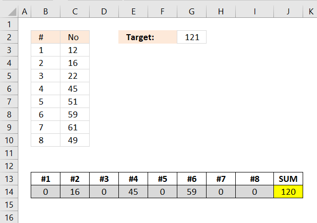
The picture shows the source numbers in cells C3:C10, eight numbers in total. They are numbered from #1 to #8 in column B. The target value is in cell G2.
The result from the formula is in cells B14 to I14 and the total is in cell J14. The combination of numbers closest to target value 121 is 16, 45, and 59 which has a total of 120. 16 + 45 + 59 equals 120.
Array formula in cell range E6:L6:
2.1 How do I enter this array formula?
- Select cell range E6:L6
- Paste the array formula in the formula bar
- Press an hold CTRL + SHIFT
- Press Enter
- Release all keys
If you did it right the formula now begins and ends with curly brackets, like this {=array formula}. They appear automatically, don´t enter the curly brackets yourself.
2.2 I want to use this formula, how do I change it?
The array formula uses this cell range $B$2:$B$9, if you need to work with more values like $B$2:$B$15 , you can change the formula following these steps.
- Copy the formula to notepad
- Press CTRL + H
- Search string $B$2:$B$9
- Replace string $B$2:$B$15
- Press with left mouse button on "Replace all" button
- Copy the formula from notepad
- Delete the old formula in excel
- Enter the new array formula in E6:Q6, see steps above.
2.3 How many numbers can I use?
If you have more than 15 numbers I recommend using my udf: Excel udf: Find positive and negative amounts that net to zero I think my udf can handle up to 20 maybe 22 values, it depends on your computer hardware.
Torstein made a great comment below: Is it possible to restrict solutions to those which have eg three numbers that adds to the total?
Yes, it is. See his question and my answer with a workbook you can get.
2.4 Explaining formula in cell E6
Step 1 - Calculate the number of combinations
The ROWS function calculates the number of rows in a cell range.
To calculate the number of combinations we can use the COMBIN function.
COMBIN(8,1) returns 8.
COMBIN(8,2) returns 28.
COMBIN(8,3) returns 56.
COMBIN(8,4) returns 70.
COMBIN(8,5) returns 56.
COMBIN(8,6) returns 28.
COMBIN(8,7) returns 8.
COMBIN(8,8) returns 1.
8+28+56+70+56+28+8+1 = 255
10 numbers return 1024 combinations.
11 numbers return 2048 combinations.
15 numbers return 32768 combinations.
20 numbers return 1048576 combinations. This is the limit, Excel can't handle arrays larger than this number. Note, VBA functions may use much larger arrays.
Instead of using the COMBIN function you can use the exponent character to calculate the number of combinations. 2 ^ 8 = 2*2*2*2*2*2*2*2 = 256. Subtract 256 with 1 and we have the number we are looking for.
INDEX($C:$C, 2^ROWS($C$3:$C$10)))
becomes
INDEX($C:$C,2^8)
2^8 is two to the power of 8 meaning 2*2*2*2*2*2*2*2 = 256
becomes
INDEX($C:$C,256)
and returns $C$256.
Step 2 - Create an array from 1 to 255
The ROW function creates a number for each cell in a cell range.
ROW($C$2:INDEX($C:$C,2^ROWS($C$2:$C$9)))-1
becomes
ROW($C$2:$C$256)-1
becomes
{2; 3; 4; 5; 6; 7; 8; 9; ... to .... ; 256}-1
and returns
{1; 2; 3; 4; 5; 6; 7; 8; ... to .... ; 255}
This array will be used to create a larger array that shows all combinations.
Step 3 - Create combination array
The INT function removes the decimal part from positive numbers and returns the whole number.
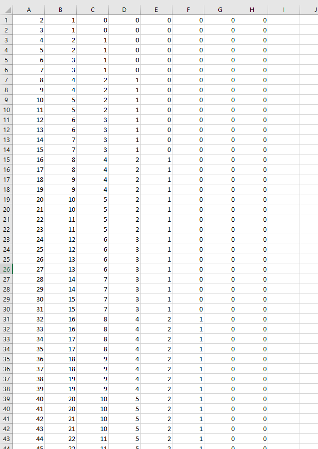
INT((ROW($C$3:INDEX($C:$C, 2^ROWS($C$3:$C$10)))-1)/2^(TRANSPOSE(MATCH(ROW($C$3:$C$10), ROW($C$3:$C$10)))-1))
This image shows the first 43 rows (out of 255 rows) of the array.
Step 4 - Create boolean array
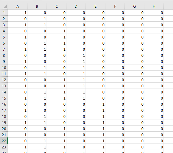
The MOD function returns the remainder after a number is divided by a divisor. This allows you to create an array that shows which numbers are valid for any given combination.
MOD(INT((ROW($C$3:INDEX($C:$C, 2^ROWS($C$3:$C$10)))-1)/2^(TRANSPOSE(MATCH(ROW($C$3:$C$10), ROW($C$3:$C$10)))-1)),2)
This image shows the first 23 rows (out of 255 rows) of the array.
Step 5 - Find total closest to target value
Calculations in step 1 to 4 are made several times in the formula, it returns an array that contains all possible combinations of the numbers used.
In this example, there are eight numbers. The calculations return an array with 255 rows and 8 columns. 255 corresponds with the number of combinations.
If I replace these calculations with the name array1 the formula becomes:
=INDEX(array1*TRANSPOSE($C$3:$C$10), MATCH(MIN(ABS(MMULT(array1, $C$3:$C$10)-$G$2)), ABS(MMULT(array1, $C$3:$C$10)-$G$2), 0), 0)
This makes it easier to understand and troubleshoot the formula. Let start with this part of the formula:
MIN(ABS(MMULT(array1, $C$3:$C$10)-$G$2))
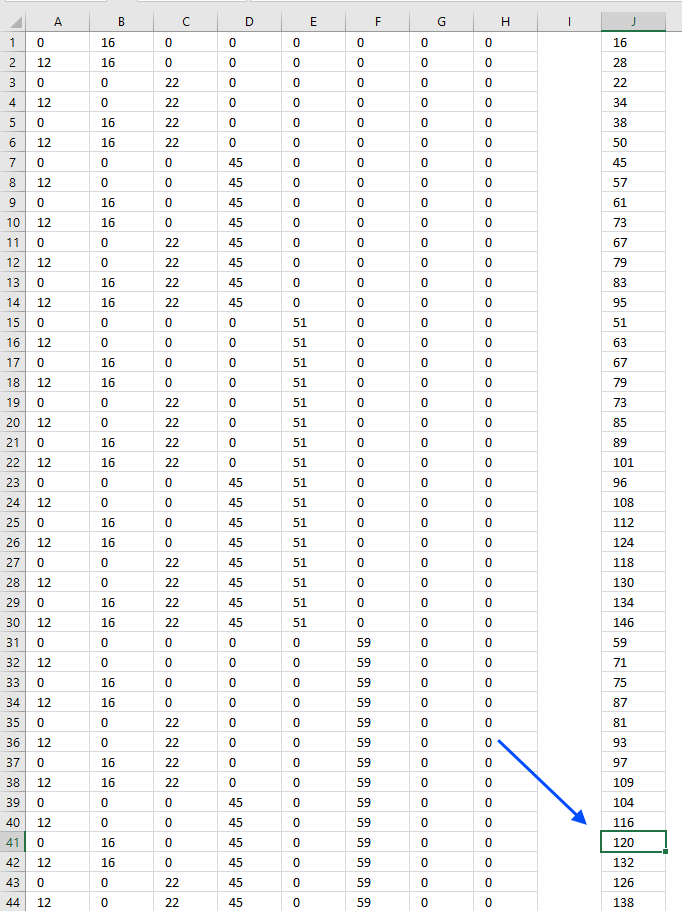
This part of the formula finds the total number that is closest to 0 (zero) meaning that number is closest to the target value. The MMULT function adds numbers on the same row and returns an array containing the totals for each combination.
MIN(ABS(MMULT(array1, $C$3:$C$10)-$G$2))
If we subtract each total with the target value we can use the MIN function to find the total that is closest to target value.
MIN(ABS(MMULT(array1, $C$3:$C$10)-$G$2))
becomes
MIN(ABS({16; 28; 22; 34; 38; 50; 45; 57; 61; 73; ... ; 315}-$G$2))
and returns 1.
Step 6 - Create array to search
We calculated this array in the previous step, however, we need to calculate this array again in order to find the position of the closest value in the array.
ABS(MMULT(MOD(INT((ROW($C$3:INDEX($C:$C, 2^ROWS($C$3:$C$10)))-1)/2^(TRANSPOSE(MATCH(ROW($C$3:$C$10), ROW($C$3:$C$10)))-1)), 2), $C$3:$C$10)-$G$2)
returns this array:
{105;93;99;87;83;71;76;64;60;48; ... ;194}
Step 7 - Find the relative position
The MATCH function returns the relative position of a given number in a cell range or array.
MATCH(MIN(ABS(MMULT(MOD(INT((ROW($C$3:INDEX($C:$C, 2^ROWS($C$3:$C$10)))-1)/2^(TRANSPOSE(MATCH(ROW($C$3:$C$10), ROW($C$3:$C$10)))-1)), 2), $C$3:$C$10)-$G$2)), ABS(MMULT(MOD(INT((ROW($C$3:INDEX($C:$C, 2^ROWS($C$3:$C$10)))-1)/2^(TRANSPOSE(MATCH(ROW($C$3:$C$10), ROW($C$3:$C$10)))-1)), 2), $C$3:$C$10)-$G$2), 0)
returns 41.
Total 120 is closest to target value 121, the chosen numbers are shown on the same row. Now we need to get those numbers and display them on the worksheet.
Step 8 - Return values
The INDEX function returns a value or multiple values based on a row and column number. IF 0 (zero) is used the entire row or column is returned.
INDEX(array1*TRANSPOSE($C$3:$C$10), MATCH(MIN(ABS(MMULT(array1, $C$3:$C$10)-$G$2)), ABS(MMULT(array1, $C$3:$C$10)-$G$2), 0), 0)
returns {0, 16, 0, 45, 0, 59, 0, 0} in cell range B14:I14. See the image below.
3. Find numbers closest to sum - Excel 365

The Excel 365 formula is 143 characters long, the earlier formula demonstrated in section 1 above is 458 characters long.
Dynamic array formula in cell B14:
It is mostly the LET function that makes this formula less than one-third in size.
4. Find numbers in total with a condition
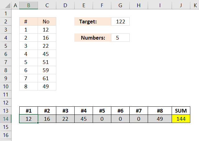
This example demonstrates a formula that selects exactly five numbers (as specified in cell G4) from the range C3:C10, ensuring their total is as close as possible to the target value in cell G2.
The result is shown in cells B14:I14, excluded numbers are represented by a 0 (zero). This example shows target value 122 and the five numbers closest to the target value are 12, 16, 22,45, and 49. Their total is 144 which is 22 from the target value 122. 122 + 22 = 144
Array formula in cell range B14:I14:
4.1 Explaining formula in cell B14
I explained the previous formula above and this formula is very similar, however, it is easier to understand the formula if I replace some calculations that are repeated several times in the formula with array1.
array1 -> MOD(INT((ROW($C$3:INDEX($C:$C, 2^ROWS($C$3:$C$10)))-1)/2^(TRANSPOSE(MATCH(ROW($C$3:$C$10), ROW($C$3:$C$10)))-1)), 2)
This formula filters rows in the array that only have the same number of items as the specified value in cell G4. The following IF function filters rows that contain the same number of items as the target value:
IF(MMULT(array1, C3:C10^0)=$G$4, ABS(MMULT(array1, $C$3:$C$10)-$G$2), "")
5. Find numbers in total with a condition - Excel 365
The image above demonstrates a formula that lets you calculate the closest target sum specified in cell G2 and how many numbers specified in cell G4.
The formula in cell B14 calculates which numbers to use, specified in cell range C3:C10, to get as close as possible to the target value using a given number of numbers.
Cell G2 contains 122 and that is the target sum, cell G4 contains 5 which is how many numbers in cells C3:C10 the formula can use. The result in cells B14:I14 show a total of 5 numbers and the sum is shown in cell J14 which is 144. This is the closest you can get to 122 using only five numbers.
Excel 365 dynamic array formula in cell B14:
The new Excel 365 LET function allows me to create a much shorter formula than the one in section 3. The formula is basically the same, however, parts that are repeated are shortened in order to improve calculations and create a smaller formula.
The LET function lets you name intermediate calculation results which can shorten formulas considerably and improve performance.
Function syntax: LET(name1, name_value1, calculation_or_name2, [name_value2, calculation_or_name3...])
Recommended reading
Which numbers add up to total? (2): Multiple Solutions
Which numbers add up to total?
Excel udf: Find positive and negative amounts that net to zero
Identify numbers in sum using solver
Find positive and negative amounts that net to zero
Find numbers in sum category
Table of Contents Identify numbers in sum using Excel solver Find numbers in sum - UDF Find positive and […]
The image above demonstrates a formula that calculates tiered values based on a tier table and returns a total. This […]
Permutations category
I discussed the difference between permutations and combinations in my last post, today I want to talk about two kinds […]
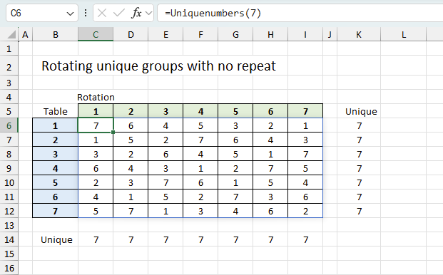
This article demonstrates ways to create unique groups with no repeat. The first example shows a formula that returns random […]
Excel categories
32 Responses to “Find numbers closest to sum”
Leave a Reply
How to comment
How to add a formula to your comment
<code>Insert your formula here.</code>
Convert less than and larger than signs
Use html character entities instead of less than and larger than signs.
< becomes < and > becomes >
How to add VBA code to your comment
[vb 1="vbnet" language=","]
Put your VBA code here.
[/vb]
How to add a picture to your comment:
Upload picture to postimage.org or imgur
Paste image link to your comment.
Thanks, Oscar!
Looks like you've managed to successfully amend the formula for this new condition (though what have you done with my Defined Names? :-)) Anyway, good work!
Also, I like the fact that you've replaced the ROW/INDIRECT constructions in my solution with the preferred ROW/INDEX ones. I myself am using this version now, though I haven't got the time to go back into all of my old posts and update them all!
Nice-looking site, by the way.
Keep up the good work.
Regards
XOR LX,
Thank you!
though what have you done with my Defined Names? :-))
Perhaps it is easier to use defined names, I don´t know. It sure makes the formula look smaller but I want to reveal the truth. ;-)
Hi Oscar and XOR LX!
I'm really impressed what you guys can do with excel formulas. I have been trying to figure out permutations for so long, but have not been able to make it.
One question to the formulas: Is it possible to restrict solutions to those which have eg three numbers that adds to the total?
Hope I make my self understood!
Regards Torstein
Torstein,
Thanks!
This sheets allows you to specify the number of values you want, cell J1. If the target value is equal to the sum, cell M6 is formatted yellow. If not equal, cell M6 is colored red.
I am sure this formula can be made smaller but I don´t know how to build a permutations array that only uses three out of 8 values, I leave that to XOR LX. :-)
Get the Excel *.xlsx file
Find numbers which are closest to a total_permut.xlsx
"I am sure this formula can be made smaller but I don´t know how to build a permutations array that only uses three out of 8 values, I leave that to XOR LX. :-)"
That's precisely what I'm looking into now!
Interesting exercise in itself.
Bear with me!
Cheers
XOR LX,
Thanks for looking in to that, I am very interested.
Done!
https://excelxor.com/2015/02/10/which-numbers-add-up-to-total-2-multiple-solutions/
Haven't yet managed to reduce the required array of zeroes and ones, so queried it with a further IF clause. More resource, I'm afraid, though not a great deal by the looks of it. Functions quite nicely, actually. :-)
I'll keep looking into ways in which we may be able to generate such reduced arrays, though. Interesting mathematical exercise!
Enjoy for now!
Thanks so much for this fantastic post!
Is there a way to find closest combination greater than or equal to the target value?
Evgeny
Thanks, yes there is.
https://www.get-digital-help.com/wp-content/uploads/2015/02/Find-numbers-which-are-equal-or-above-to-a-total.xlsx
Hi Oscar,
This is exactly what I've been looking for...
I just want to add an extra rule into this formula that would exclude all the values that are higher than 260. Are you able to help me with this extra requirement?
Thanks in advance and congrats for sharing your knowledge.
JRM
Thanks so much for this fantastic post!
Is there a way to do this for more data? I sometime need it for more that 100 items.
Thanks in advance and congrats for sharing your knowledge.
thanks oscar, awesome post as always.
1 question: can the array formula work in vertical format, at column C2:C9?
this would be helpful when the list has other information.
lohhw3,
Thank you. Yes, you can.
1. Select cell range C2:C9
2. Enter the same array formula in the formula bar, except use transpose function around the entire array formula, like this:
=TRANSPOSE(arrayformula)
3. Press Ctrl + SHIFT + ENTER
Thanks for this! I saw you offered a version for a combination greater than or equal to the target. I'd really appreciate it if you could show me how to go about changing it to be LESS than or equal to the target. I fiddled around with it for a while but it's beyond me.
SC,
I think I got it working.
Find-numbers-which-are-equal-or-less-than-target-value.xlsx
Hi Oscar,
This is amazing, and incredibly interesting. Couple of quick questions, would there be a way to change the formally so you can both pick the amount of numbers in the solution and also only find a solution that's greater than your number. Also, would there be a way to have the formula also look at having multiples of one number if that is closer than any pother combination (e.g. if I had 1,3,20,30 and I want to get to 26 using 3 numbers it would spit out two 3's and one 20 instead of one 1, one 3, and one 20). Really appreciate your hard work putting this together.
Josh Cohen,
Would there be a way to change the formally so you can both pick the amount of numbers in the solution and also only find a solution that's greater than your number.
Try this workbook.
Find-numbers-which-are-closest-to-a-total2.xlsx
Also, would there be a way to have the formula also look at having multiples of one number if that is closer than any other combination (e.g. if I had 1,3,20,30 and I want to get to 26 using 3 numbers it would spit out two 3's and one 20 instead of one 1, one 3, and one 20)
I believe you need a custom function to do that.
Hi Oscar, I believe the total2.xlsx workbook formula doesn't work exactly as intended.
Two things I noted, cases: Fix numbers to be used = 3:
- The combinations found don't just include numbers that are "greater" than your target number but also which are equal to that, try for example 124 (or 122) for which an exact match is provided --> output = 16+59+49=124
- The results also seem to include closest matches that are LOWER than the target value, for example: target = 123 --> output = 22+51+49 = 122 which seems to be an unexpected result?
Is there a way to tweak the formula to work correctly?
Further I was wondering whether there's a way to determine the number of possibilities that yield the desired target result: e.g. a target value of 124 could be achieved from 3 numbers in at least the following 2 ways:
1) 12+51+61 = alternative solution not provided by formula
2) 16+49+59 = formula solution
Many thanks and Best Regards
René, you are right. There was a problem with the formula. I found the error and it seems to work fine now.
Find-numbers-which-are-closest-to-a-total3.xlsx
Rene,
Further I was wondering whether there's a way to determine the number of possibilities that yield the desired target result: e.g. a target value of 124 could be achieved from 3 numbers in at least the following 2 ways:
1) 12+51+61 = alternative solution not provided by formula
2) 16+49+59 = formula solution
Interesting question. Yes, it is possible. See this workbook:
Find-numbers-which-are-closest-to-a-total5.xlsx
OP,
First of all thank you so much. You have no idea. I have been trying to figure out for quite some while now, without using solver or any "push button" or "activation" method, to do this with just two numbers but multiple times.
So to help this poster out, what I did was define my first two numbers and then the next 12 rows I had them alternate to equal the original two rows. So with a total of 14 rows I could have 7 possible of each two numbers to get closest to the target number. Obviously if you need more then two original numbers then that starts to eat into your possible scenarios.
Now OP if you could help me with one issue that I have had with implementing this formula. With the INDEX Column reference B:B, it does not follow me when I cut/paste to another location/worksheet/workbook. I really need this formula in the final form I get it to be able to just cut/paste into various workbooks and then once in the workbook I define those two values and the target value and then I am done. Is there another way to do the column reference so that it follows you?
Also back to your answer to this poster on the multiples, if you did do a function for the multiples instead would it be possible to make it easily copied across workbooks or would someone need to know what they are doing?
What I am trying to do is create something for many individuals that know little about excel so I am trying to keep it as simple as possible for them to copy over and maybe define a few cells.
Thank you
Thank you, I really appreciate this. This is my very first time using excel and "Find numbers closest to sum" was a daunting task... I really appreciate the step by step way that you did this, people must forget that they had a first time and no matter how hard they try they always leave something out of their description and that really is a downer. (You didn't put the step in about how to sum everything at the end, but I figured it out after 2 or 3 hours). Thanks again..
I have a similar problem with an Array of as many as 26 rows and 6 columns.
Is there a way to adapt this so that is selects one number form each row
such that the sum of that row adds up to as close to the target as possible.
Then does the same for all 26 rows. So that no 2 values are repeated,
and the sum of each row is as close as possible to the (Target) Mean sum of all rows?
Hi Oscar, During first paste I'm getting error like: The formula you pasted contains an error.
=INDEX(MOD(INT((ROW($C$3:INDEX($C:$C, (...)
I got $C:$C reference highlighted.
Any thoughts?
Thanks in advance!
if ı have numbers at 4 columns and 50 rows. How to find combinations that closest given sum in Excel?
Thanks so much Oscar. it is impressive post.
Is there a way to find closest combination but finding sum can be low target value?
and also if ı have 5 columns and 10 rows, can ı calculate it like this?
Hola, primero felicitarle por su pagina web, que es de mucha ayuda para la humanidad. Luego, le informo que el archivo de Excel, del articulo: Autor: Oscar Cronquist Artículo actualizado en Junio 09, 2022: Encuentra los números más cercanos a la suma, no se puede descargar, al intentar de descargar sale una página de error. Le agradecería que por favor suba el archivo de nuevo para poderlo descargar. Gracias.
Thanks Oscar, awesome
Can the new functions in Excel 2021 make this formula simpler?
Ali,
I think you missed the Excel 365 formula above?
https://www.get-digital-help.com/find-numbers-closest-to-sum/#2
If not, I'll create a new Excel 365 formula for the third section: Find numbers in total with a condition the coming days.
Thanks so much for this great post!
i need it with a way to do this for more data & amounts ? I need it for 1000 items. if you could do it, it will help with my manager at work please i need your help .
Thanks in advance .
Hi Emma,
It is a very cpu intensive task, the limit is somewhere between 20 to 30 numbers. The number of combinations become quickly incredibly large.
Hi Oscar,
I always appreciate your website for special formulas.
Now I wanted to simplify the more complicated formula from ‘...total5.xlsx’ with a LET formula for the range D10:D17 – but the formula is giving me incorrect results!
Where do I need to adjust the basic formula?
Best regards
Adrian