Working with running totals
Andrew asks:
LOVE this example, my issue/need is, I need to add the results. So instead of States and Names, I have to match a client name, and add all the sales totals:
clientA 10
clientA 10
clientA 10
clientB 5
clientB 5
clientB 5
So if I search for clientA, I need one cell that keeps a running total as sales are added. Lastly, a date range will need to be given, so search for sales from clientA between two dates and keep a running total...
Table of Contents
1. Running totals based on criteria - formula

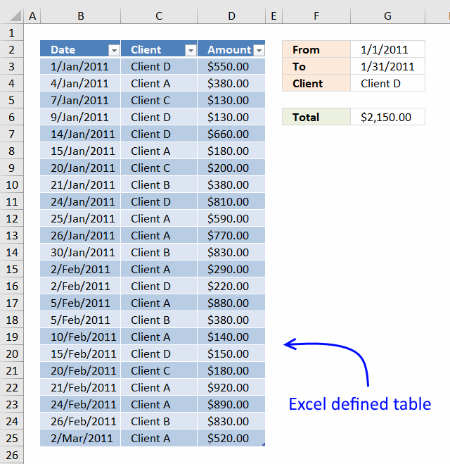
The image above demonstrates a formula in cell E3 that calculates a running total based on a date range specified in cells H2, H3, and a condition specified in cell H4.
Formula in cell E3:
Explaining the formula in cell E3
Step 1 - Populate SUMIFS function arguments
The SUMIFS function adds numbers based on criteria.
Function syntax: SUMIFS(sum_range, criteria_range1, criteria1, [criteria_range2], [criteria2], ...)
sum_range - $D$3:D3
criteria_range1 - $C$3:C3
criteria1 - $H$4
[criteria_range2] - $B$3:B3
[criteria2] - "<="&$H$3
[criteria_range3] - $B$3:B3
[criteria3] - ">="&$H$2
Cell reference $D$3:D3 contains an absolute part $D$3 indicated by the dollar signs and a relative part D3. This makes the cell reference grow when the cell is copied to the cells below.
This is also the case with $C$3:C3 and $B$3:B3, this makes the formula include more and more cells in columns B, C, and D creating the running total effect.
The less than, greater than, and equal sign shown in "<="&$H$3 and ">="&$H$2 let you create a condition so that the date range criteria are met.
The third condition is specified in cell $H$4, it makes sure that the running total is only valid for "Client D".
SUMIFS(sum_range, criteria_range1, criteria1, [criteria_range2], [criteria2], [criteria_range3], [criteria3], ...)
becomes
SUMIFS($D$3:D3,$C$3:C3,$H$4,$B$3:B3,"<="&$H$3,$B$3:B3,">="&$H$2)
Step 2 - Evaluate SUMIFS function
SUMIFS($D$3:D3,$C$3:C3,$H$4,$B$3:B3,"<="&$H$3,$B$3:B3,">="&$H$2)
returns 550.
2. Running totals based on criteria - formula and Excel Table

I highly recommend a pivot table for this task, however, this article demonstrates a formula combined with an Excel defined table. A pivot table is lightning fast if you have lots of data to work with and is easy to learn.
The Excel Table is great for a list that keeps growing, the references to the Excel Table don't change which makes the formula easy to use. There is no need to adjust cell references, they are called structured references and are only used in Excel Tables.
This example shows how to calculate a running total using a formula based on a date range and a condition. This example is different from the one in section 1, it calculates a total for all data in the Excel Table. You can add more data to the Excel Table and the formula adjusts automatically creating a running total.
Formula in cell G6:
The SUMIFS function was introduced in Excel 2007, use the SUMPRODUCT function if you have an earlier Excel version.
How to create an Excel defined table
- Select a cell in the data set.
- Press CTRL + T
- A dialog box appears, enable checkbox if your data set has headers.
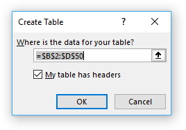
- Press with left mouse button on OK.
Explaining the formula in cell G6
Some of the cell references in the SUMIFS function are structured references pointing to a range in an Excel defined table. Structured references adjust automatically when data is added or removed to the table, the formula will instantly return the new running total.
Structured reference -> Table1[Amount]
The SUMIFS function adds numbers based on criteria and returns the total.
SUMIFS(sum_range, criteria_range1, criteria1, [criteria_range2], [criteria2], ...)
Step 1 - First argument is sum_range
The sum_range argument is a structured reference: Table1[Amount]. This cell range contains the numbers to be added based on criteria.
Step 2 - Second and third argument
The first pair of arguments evaluates if cells in column Client equal value in cell G4.
| Argument | Cell reference |
| criteria_range1 | Table1[Client] |
| criteria1 | G4 |
Step 3 - Fourth and fifth argument
The second pair of arguments evaluates if cells in column Date are equal or are less than value in cell G3.
| Argument | Cell reference |
| criteria_range2 | Table1[Date] |
| criteria2 | "<="&G3 |
The less than and equal signs are concatenated to cell reference G3 using the ampersand character.
Step 4 - Sixth and seventh argument
The third pair of arguments evaluates if cells in column Date are equal or are larger than the value in cell G2.
| Argument | Cell reference |
| criteria_range3 | Table1[Date] |
| criteria3 | ">="&G2 |
The larger than and equal signs are concatenated to cell reference G2 using the ampersand character.
3. Get the Excel file
4. Running totals based on criteria - Excel Table

This example shows how to calculate a running total using an Excel Table only based on a date range and a condition.
Excel 2007 and later versions let you add a total row below the Excel Table. Here is how to enable the total row:
- Select any cell in the Excel Table.
- A new tab on the ribbon appears named "Table Design", press with left mouse button on that tab to select it.
- Press with mouse on the "Total row" check box to enable it.

The total row is now visible.
4.1 How to filter an Excel Table

The Excel Table has small buttons containing an arrow next to the column header names. Press with mouse on the button next to "Date".

A popup menu appears, deselect all checkboxes except "January".

Press with left mouse button on the "OK" button.

Note, the button next to the column header name "Date" has changed, and the new icon tells you that a filter is present.
Press with left mouse button on the button next to the column header name "Client", and a popup menu appears.

Deselect all check boxes except "Client D", then press with left mouse button on the "OK" button.

4.2 How to clear an Excel Table filter
Press with left mouse button on the button next to the column header name you want to clear, a popup menu appears.

Press with left mouse button on "Clear Filter From "Date".

5. How to create running totals
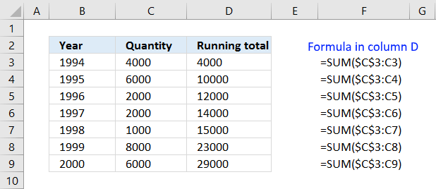
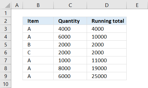
This article demonstrates a formula that calculates a running total. A running total is a sum that adds new numbers to the total as you copy the formula to cells below.
The image above shows numbers in column C, the formula in cell D3 adds the number in cell C3 and returns the total which is 4000.
Cell D4 adds the number in cell C3 and cell C4 and returns 10000 which is the result of 4000 + 6000. Cell D5 returns 12000 which is the sum of 4000 + 6000 + 2000 equals 12000.
I also demonstrate running totals formulas that adds values based on a condition, based on month, and when the date changes to a new month.
What's on this page
- Create a formula that returns running totals
- Running totals with a condition
- Running totals on a monthly basis
- Display a running total when the month changes
- Get Excel *.xlsx file
5.1. Create a formula that returns running totals
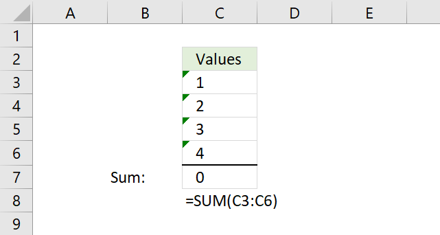
The SUM function in cell D3 uses only a single cell reference and still manages to sum current and previous values in column D. Read on to find out how.
The formula in cell D3:
5.1.1 Explaining formula
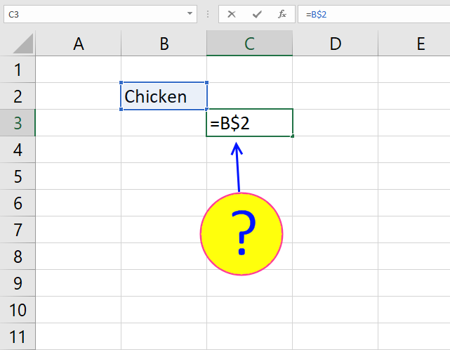
Step 1 - Cell reference
$C$3:C3
The SUM function has a cell reference that consists of two parts, the first part has a dollar sign before the column character and another one before the row number.
The dollar sign tells you that the cell reference is locked and won't change if you copy the formula. In Excel terminology: an absolute cell reference.
However, the second part of the cell reference has no dollar signs, and that part changes when you copy and paste the formula to other cells. In Excel terminology: a relative cell reference.
What happens when you copy the cell and paste it to cell D4?
The second part of the cell reference now points to cell C4 and the first part is still pointing to cell C3. The cell reference expands as you copy the formula to cells below.
If you want to learn more about absolute and relative cell references, read the following article:
Recommended articles
What is a reference in Excel? Excel has an A1 reference style meaning columns are named letters A to XFD […]
Step 2 - Add numbers
The SUM function adds numbers in a cell range or array and returns a total.
SUM($C$3:C4)
becomes
SUM(4000; 6000)
and returns 10000.
5.2. Running totals with a condition
The formula above in column D calculates running totals based on a condition. The condition changes depending on the value in column B on the same row as the formula.
Example 1, in cell D6 the formula calculates the sum for Item C. Item C is only in cell B6, the corresponding value in column C is B6. The formula returns 2000 in cell D6.
Example 2, in cell D7 the formula calculates the sum for Item A. Item A is in cell B3, B4 and B7, the corresponding values in column C are C3,C4 and C7.
4000 + 6000 + 1000 = 11000
The formula returns 11000 in cell D7. There are several ways to calculate a running total based on a condition, the easiest and smallest formula is probably the SUMIF function.
Formula in cell D3:
5.2.1 Explaining formula in cell D9
The arguments in a SUMIF function are: SUMIF(range, criteria, [sum_range])
The range argument grows when the formula is copied to cells below. $B$3:B3 changes to $B$3:B4 when the formula is copied to cell D4. This applies to the [sum_range] argument as well.
The expanding cell references make this formula include more and more cells and allowing it to calculate running totals based on a condition.
SUMIF($B$3:B9,B9,$C$3:C9)
becomes
SUMIF({"A"; "A"; "B"; "C"; "A"; "A"; "A"},"A", {4000; 6000; 2000; 2000; 1000; 8000; 6000})
and returns 25000. 4000 + 6000 + 1000 + 8000 + 6000 equals 25000.
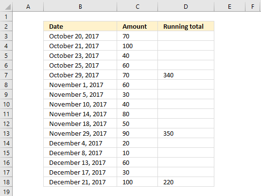
5.3. Running totals on a monthly basis
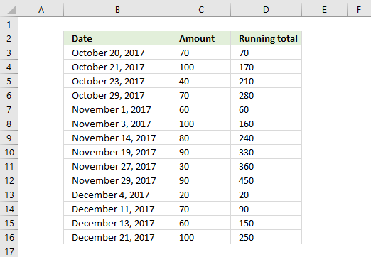
This example demonstrates how to create a formula that returns a running total based on the month specified on the same row as the formula.
The dates in column B must be sorted in ascending or descending order for this formula to work appropriately.
Formula in cell D3:
The dates in column B are sorted in ascending order, however, the formula works fine for dates sorted in descending order as well.
The formula in column D adds amounts to a running total using the corresponding date as a condition.
Example, the formula in cell D6 uses this text string "2017-10" in cell B6 as a condition to add all previous amounts above cell D6 that also return text string "2017-10".
In other words, the formula creates a running total for the current month and starts all over when a new month begins.
5.3.1 Explaining formula in cell D8
Note that I am explaining the formula in cell D8, not cell D3.
Step 1 - Convert corresponding date to a text string
TEXT(B8, "YYYY-MM") returns 2017-11
In this case, the TEXT function converts a date to a particular format specified in the second argument. YYYY returns the year and MM returns the month number.
Step 2 - Convert corresponding dates to text strings
TEXT($B$3:B8, "YYYY-MM") returns the following array {"2017-10";"2017-10";"2017-10";"2017-10";"2017-11";"2017-11"}
The first argument in the TEXT function is a cell range containing multiple values. The TEXT function returns an array with the exact same number of values.
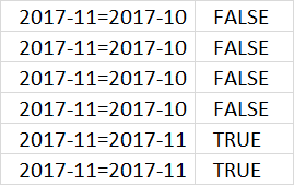
Step 3 - Build a logical expression
TEXT(B8, "YYYY-MM")=TEXT($B$3:B8, "YYYY-MM")
becomes
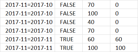
2017-11={"2017-10";"2017-10";"2017-10";"2017-10";"2017-11";"2017-11"}
and returns {FALSE; FALSE; FALSE; FALSE; TRUE; TRUE}
Step 4 - Multiply with amounts
(TEXT(B8, "YYYY-MM")=TEXT($B$3:B8, "YYYY-MM") )*$C$3:C8
becomes
{FALSE; FALSE; FALSE; FALSE; TRUE; TRUE}*{70;170;210;280;60;160;240}
and returns {0; 0; 0; 0; 60; 100}
Step 5 - Sum values
SUMPRODUCT((TEXT(B3, "YYYY-MM")=TEXT($B$3:B3, "YYYY-MM"))*$C$3:C3)
becomes
SUMPRODUCT({0; 0; 0; 0; 60; 100})
and returns 160 in cell D8.
Recommended article:
Recommended articles
Andrew asks: LOVE this example, my issue/need is, I need to add the results. So instead of States and Names, […]
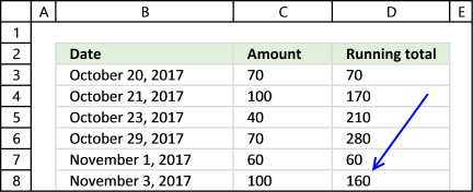
5.4. Calculate a running total when the month changes
Formula in cell D3:
The picture above shows a formula in column D that shows the running total if the next cell in column B contains a new month.
Explaining formula in cell D7
Note, I will explain the formula in cell D7. The cell references have changed, the formula now looks like this:
Why will I explain the formula in cell D7? Not much is happening in D3, D4, D5 and D6.
Step 1 - Check if month is not equal to month in cell below
In this example, the TEXT function converts a date to a particular format specified in the second argument. YYYY returns the year and MM returns the month number.
TEXT(B7, "YYYY-MM")<>TEXT(B8, "YYYY-MM")
becomes
"2017-10"<>"2017-11"
and returns TRUE.
Step 2 - Convert corresponding date to a text string
TEXT(B7, "YYYY-MM") returns 2017-10
Step 3 - Convert corresponding dates to text strings
TEXT($B$3:B7, "YYYY-MM") returns the following array {"2017-10";"2017-10";"2017-10";"2017-10";"2017-10"}
The first argument in the TEXT function is a cell range containing multiple values. The TEXT function returns an array with the exact same number of values.
Step 4 - Build a logical expression
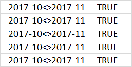
TEXT(B7, "YYYY-MM")=TEXT($B$3:B7, "YYYY-MM")
becomes
2017-10={"2017-10";"2017-10";"2017-10";"2017-10";"2017-10"}
and returns {TRUE; TRUE; TRUE; TRUE; TRUE}
Step 5 - Multiply with amounts
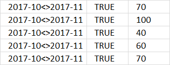
(TEXT(B7, "YYYY-MM")=TEXT($B$3:B7, "YYYY-MM") )*$C$3:C7
becomes
{TRUE; TRUE; TRUE; TRUE; TRUE}*{70;100;40;60;70}
and returns {70;100;40;60;70}
Step 6 - Sum values
SUMPRODUCT((TEXT(B7, "YYYY-MM")=TEXT($B$3:B7, "YYYY-MM"))*$C$3:C7)
becomes
SUMPRODUCT({70;100;40;60;70})
and returns 340 in cell D8.
5.5 Get Excel *.xlsx file
Sum category
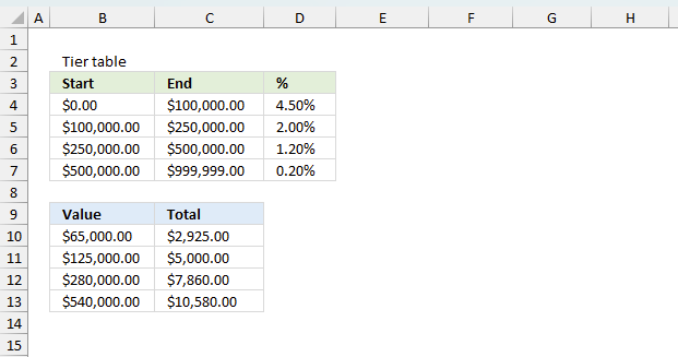
The image above demonstrates a formula that calculates tiered values based on a tier table and returns a total. This […]
This article explains why your formula is not working properly, there are usually four different things that can go wrong. […]
Excel categories
9 Responses to “Working with running totals”
Leave a Reply
How to comment
How to add a formula to your comment
<code>Insert your formula here.</code>
Convert less than and larger than signs
Use html character entities instead of less than and larger than signs.
< becomes < and > becomes >
How to add VBA code to your comment
[vb 1="vbnet" language=","]
Put your VBA code here.
[/vb]
How to add a picture to your comment:
Upload picture to postimage.org or imgur
Paste image link to your comment.
Oscar,
Thank you so much!!!! Not only did this solve my issue, I have now learned a lot more about these functions to use on future projects.
Your site is a fabulous resource!!
Thank you again.
~Andrew
i think using only sumproduct formula too easy..
=SUMPRODUCT((B3:B25>=F3)*(B3:B25<=G3)*(C3:C25=H3)*(D3:D25))
mustafa,
The cell references have to be expanding as new records are added, in order to keep a running total.
Hello again Oscar,
I am playing with this some more, and I using the Microsoft Date and Time Picker (Excel 2010) to use for the two dates. I appear to have all the dates matching (dd/mm/yyyy) on both the PO list and my date range cells. However, the formula doesn't seem to be using the dates anymore?
Any thoughts?
Thanks.
~Andrew
Andrew Matheson,
Send me an excel file without sensitive information: Contact me
and I´ll se what I can do.
Looks like an easy pivot table solution to me.
David Hager,
As far as I know, pivot tables are not dynamically updated when new values are added.
The SUMPRODUCT function is easy to understand, it´s the dynamic ranges that make it look complicated.
Now I know: How to create a dynamic pivot table and refresh automatically in excel
For above example how to get date when for client d total exceeded $1200 through formula without helper cells.
Thanks