Use VLOOKUP to calculate discounts, commissions, tariffs, charges, shipping costs, packaging expenses or bonuses

Have you ever tried to build a formula to calculate discounts based on price? The VLOOKUP function is much easier to use than nested IF functions.

You can also use the methods described in this article to calculate commissions, tariffs, charges, shipping costs, packaging expenses etc.

I wrote an article on how to calculate tiered values based on a tier table, however, you can't use the VLOOKUP function in those calculations as far as I know.

1. Introduction

What are discounts? Discounts are price reductions that make things cheaper. Bigger orders often get bigger discounts. Example:

Buy 1 item → No discount
Buy 10 items → 10% discount
Buy 50 items → 20% discount

What is a commission? A commission is money paid to a person for selling something. Salespeople may earn different commissions based on total sales. Example:

Sell $1,000 worth → 5% commission
Sell $5,000 worth → 10% commission

What are tariffs? Tariffs are taxes on goods coming from other countries. Some tariffs depend on quantity or value. Example:

Small imports may have low tariffs
Large imports may have higher tariffs

What are charges? Charges are extra costs for services or products. Service fees may change based on usage. Example:

Bank transfer below $100 → $2 charge
Bank transfer above $500 → No charge

What are shipping costs? Shipping costs are the money paid to send goods from one place to another. Shipping gets cheaper per item when buying more. Example:

Ship 1 item → $5
Ship 10 items → $20 ($2 per item)

What are packaging expenses? Packaging expenses are the costs of wrapping and protecting goods before selling or shipping. Costs may go down for large orders. Example:

1 box costs $3
100 boxes cost $200 ($2 per box)

What are bonuses? A bonus is extra money for good work.

Quantity-Based Bonuses – More purchases or sales can lead to bigger bonuses. Example:

Sell 10 items → $10 bonus
Sell 50 items → $100 bonus

Total Cost-Based Bonuses – Higher spending or revenue earns better rewards. Example:

Spend $500 → Get a $20 bonus
Spend $1,000 → Get a $50 bonus

Tier-Based Bonuses – Different levels offer different rewards. Example:

Bronze tier (sales below $1,000) → 2% bonus
Silver tier (sales above $1,000) → 5% bonus
Gold tier (sales above $5,000) → 10% bonus

2. How do I use different price ranges to determine a discount?

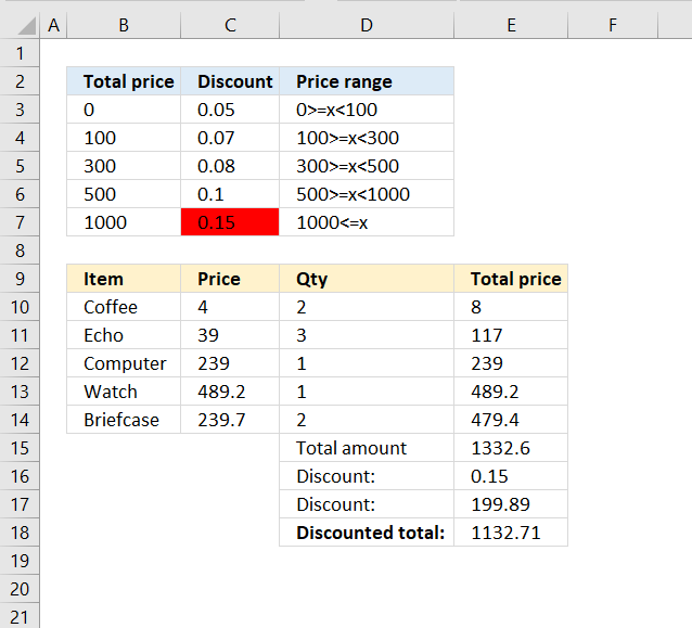
For this example our price range plan looks like this:

• Total price between 0 and 100 returns a 5% discount
• Total price between 100 and 300 returns a 7% discount
• Total price between 300 and 500 returns an 8% discount
• Total price between 500 and 1000 returns a 10% discount
• Total price between 1000 and above returns a 15% discount

The picture above shows you the discount percentage table (B2:D7) and a summary table (B9:E19) with a calculated discount (E21).

The table above shows you the total amount of all items $1 332.60 in cell E20, the formula in cell E21 calculates a discount percentage. Since $1 332.60 is larger than $1 000 the formula returns 15%.

Cell E23 returns the discounted total.

Keep in mind, the values in the first column (B3:B7) must be sorted ascending. The third column (D3:D7), dhown in the image above, is not necessary for the formula calculation.

Formula in cell E21:

Formula in cell E22:

Formula in cell E23:

The following chart shows you the different discount ranges from table above.

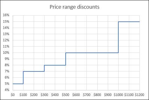
Read on to learn more about linear discounts.

Back to top

3. How do I calculate a discount based on a linear equation?

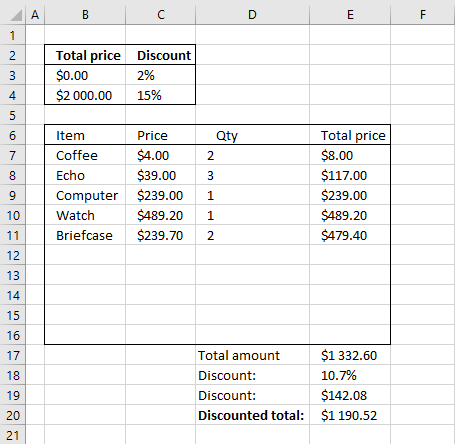
In this scenario, we want to use a linear equation to calculate the discount percentage. It begins on 0 (zero) with 2% and climbs up to 15% on $2 000, shown in cell range B3:C4 on the picture below.

These four numbers are our two coordinates. A coordinate in a plane has two values, x, and y. You can draw a line between two coordinates thus a linear equation.

Formula in cell E18:

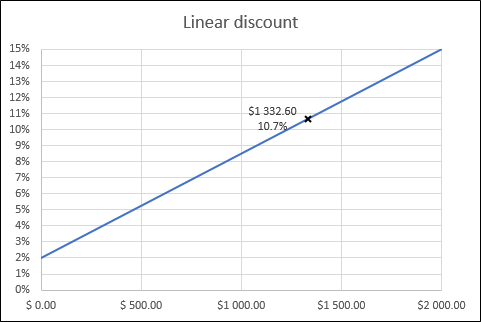
You can verify the calculated discount value by looking at this chart.

3.1 What is the formula in cell E18 doing?

It calculates the discount based on a linear equation. A linear equation looks like this:

where k and m are constants.

Constant k is the slope of the line, the line slants from left to right if k is negative. Constant m is the y-coordinate where the line crosses the y-axis.

A linear equation consists of two coordinates (x1, y1) and (x2, y2). In this example, shown in the image above, the coordinates are: (0,0.02) and (2000,0.15). This means that the discount starts at 2% and increases to 15% when the value is 2000.

Step 1 - How to calculate constant k in a linear equation?

To determine constant k we need to know two coordinates on the line.

k is calculated like this: (y2-y1)/(x2-x1) or if we use the actual cells on the worksheet: (C4-C3)/(B4-B3). Variable x is the total amount, calculated in cell E17.

Step 2 - How to calculate constant m in a linear equation?

y=kx+m

m is called the y-intercept meaning m equals y if x is zero. This is what we get if we use cells on the worksheet: C3-((C4-C3)/(B4-B3))*B3

Step 3 - Calculate discount based on price

We now know how to calculate k and m, we can now build the linear equation.

y = kx + m becomes  (C4-C3)/(B4-B3)*E17+C3-((C4-C3)/(B4-B3))*B3

Evaluate formula in cell E18

Step 1 - Calculate the slope of the line

(C4-C3)/(B4-B3)

becomes

(0.15-0.02)/(2000-0)

The parentheses allow us to control the order of calculations, we want to subtract before we divide.

(0.15-0.02)/(2000-0)

becomes 0.13/2000 and returns 0.000065.

Step 2 - Calculate the y-intercept

C3-((C4-C3)/(B4-B3))*B3

becomes 0.02-((0.15-0.02)/(2000-0))*0 becomes

0.02-0 and returns 0.02

Step 3 - Calculate equation

y=kx+m

(C4-C3)/(B4-B3)*E17+C3-((C4-C3)/(B4-B3))*B3

becomes 0.000065*E17+0.02 becomes 0.000065*1332.6+0.02 and returns 0.106619.

Back to top

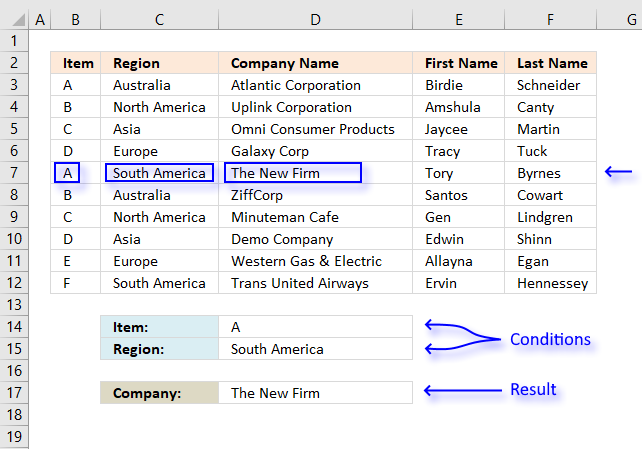
4. How can I use multiple tables to calculate a discount based on different price levels?

This example demonstrates how to use two different tables. The discount percentage depends on the category, the first table is category A and the second table is category B.

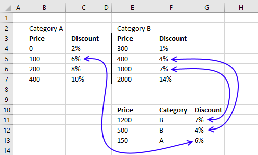
Formula in cell G11:

Back to top

4.1 Explaining function in cell G11

You can easily follow the formula calculations, step by step.

1. Select cell G11.
2. Go to tab "Formulas" on the ribbon.
3. Press the "Evaluate formula" button.

Press on the "Evaluate" button to see the next step in the calculation, press with left mouse button on OK when done.

Step 1 - Identify the relative position of category in array

MATCH(F11,{"A","B"},0)  returns 2.

B is the second number in the array {"A","B"}. In other words, the MATCH function converts the category to a number. The number determines which range to be used.

Step 2 - Choose cell range

INDEX(($B$4:$C$7,$E$4:$F$7),,,MATCH(F11,{"A","B"},0)) returns $E$4:$F$7.

The INDEX function returns cell range $B$4:$C$7 or $E$4:$F$7 depending on the category. An entire range is returned because both row and column parameters are omitted.

Step 3 - Use cell range in VLOOKUP function and return the corresponding discount percentage

VLOOKUP(E11,INDEX(($B$4:$C$7,$E$4:$F$7),,,MATCH(F11,{"A","B"},0)),2,TRUE)

returns 7%.

The VLOOKUP function uses the selected range to retrieve the discount value from column 2 in the second table. Make sure the leftmost column in the tables are sorted descending.

Tip! This post explains how to use multiple conditions in a VLOOKUP function:
Use multiple conditions in Vlookup

Back to top

5. How do I calculate a bonus based on multiple linear equations?

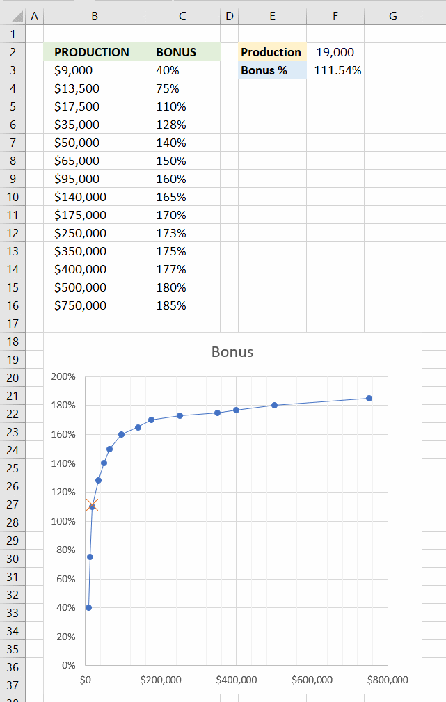
This example demonstrates how to calculate a bonus based on different ranges, the bonus is linear between the levels. Please see image above.

Simply enter a value in cell F2 and if the value falls between two levels then the formula calculates the bonus based on a linear equation on those particular levels.

The value in cell F2 is 19,000 and it falls between $17,500 and $35,000, the bonus is 110% and 128% respectively. The number is, however, between these two numbers so the formula calculates the bonus based a line between 110% and 128%.

The chart above shows the ranges and the lines between these ranges. The VLOOKUP function can't be used in this particular example.

Formula in cell F3:

4.1 Explaining formula in cell F3

The linear equation used in this example to calculate the result is y = k*x+m

Step 1 - Identify levels based on input value and bonus table

The MATCH function allows you to get the relative position of a value in a  cell range, the table is sorted from low to high.

This allows me to find the ranges that the value falls between if I use 1 in the third argument. Please see the documentation for the MATCH function if you want to read the details.

MATCH(F2, B3:B16, 1) returns 3.

Step 2 - Return values

The OFFSET function lets you return an array based on a row, column number and the size of the cell range.

OFFSET(C3, MATCH(F2, B3:B16, 1)-1, , 2) returns {17500; 35000}.

I could have used the INDEX function to accomplish the same task, however, the SLOPE function won't let me. The OFFSET function will do.

Step 3 - Calculate the slope

The equation we use is y = kx + m. k is the slope of the line. To calculate the slope we need two y values and two x values. k = (y₂-y₁)/(x₂-x₁)

The SLOPE function lets you calculate the slope using two or more coordinates.

SLOPE(OFFSET(C3, MATCH(F2, B3:B16, 1)-1, , 2), OFFSET(B3, MATCH(F2, B3:B16, 1)-1, , 2))

returns 0.0000102857.

Step 4 - Calculate where the line crosses the y axis

The equation we use is y = kx + m. m represents the value where the line crosses the y axis. x is 0 (zero).

The INTERCEPT function is handy in this case, it allows you to calculate the m value using two or more coordinates.

INTERCEPT(OFFSET(C3, MATCH(F2, B3:B16, 1)-1, , 2), OFFSET(B3, MATCH(F2, B3:B16, 1)-1, , 2))

becomes

INTERCEPT({1.1; 1.28}, {17500; 35000})

and returns 0.92.

Step 5 - Calculate bonus

F2*SLOPE(OFFSET(C3, MATCH(F2, B3:B16, 1)-1, , 2), OFFSET(B3, MATCH(F2, B3:B16, 1)-1, , 2))+INTERCEPT(OFFSET(C3, MATCH(F2, B3:B16, 1)-1, , 2), OFFSET(B3, MATCH(F2, B3:B16, 1)-1, , 2))

becomes

19000*0.0000102857 + 0.92

and equals 1.1154283 (111.54%).

Get the Excel file

Production-Bonusv5.xlsx

6. How to perform two-way lookup in multiple tables

This example shows you how to do lookups in multiple tables.

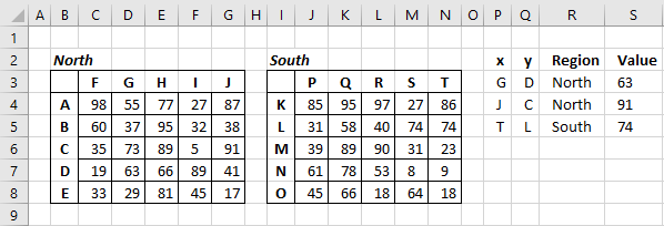
Formula in cell S3:

Back to top

5.1 Explaining formula in cell S3

The INDEX function allows you to choose between different cell ranges depending on the region value in cell R3, if a value is present in the optional parameter area_num.

You can easily follow the formula calculations, step by step.

1. Select cell S3
2. Go to tab "Formulas" on the ribbon
3. Press with left mouse button on "Evaluate formula" button

Press with mouse on "Evaluate" button to see next step in the calculation, press with left mouse button on OK when done.

Step 1 - Identify which cell range to fetch data from, C4:G8 or J4:N8

The MATCH function lets you find out where in an array a value is located (relative position).

INDEX(($C$4:$G$8,$J$4:$N$8),,,MATCH(R3,{"North","South"},0))

becomes

INDEX(($C$4:$G$8,$J$4:$N$8),,,1,0))

and returns the first cell reference $C$4:$G$8.

Step 2 - Identify which cell range to search in, B4:B8 or I4:I8

INDEX(($B$4:$B$8,$I$4:$I$8),,,MATCH(R3,{"North","South"},0))

returns $B$4:$B$8

Step 3 - Match value "D" in cell range $B$4:$B$8

MATCH(Q3,INDEX(($B$4:$B$8,$I$4:$I$8),,,MATCH(R3,{"North","South"},0)),0)

returns 4. Now we know the row number to use.

Step 4 - Find column number

The steps to look for the column number is almost identical to finding the row number.

MATCH(P3,INDEX(($C$3:$G$3,$J$3:$N$3),,,MATCH(R3,{"North","South"},0)),0)

returns 2.

Step 5 - Return value from intersection of a row and column number

INDEX(INDEX(($C$4:$G$8,$J$4:$N$8),,,MATCH(R3,{"North","South"},0)),MATCH(Q3,INDEX(($B$4:$B$8,$I$4:$I$8),,,MATCH(R3,{"North","South"},0)),0),MATCH(P3,INDEX(($C$3:$G$3,$J$3:$N$3),,,MATCH(R3,{"North","South"},0)),0))

returns 63.

You can easily modify the formula to search simultaneously in 4 different cross reference tables.

Example:

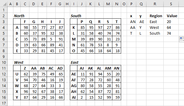
Formula in cell S3:

Tip! Read this post to do Reverse two-way lookup in a cross reference table.

Back to top

Get the Excel file

VLOOKUP-discount-percentagesv2.xlsx

Back to top

Two dimensional lookup category

How to perform a two-dimensional lookup
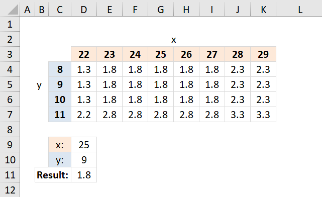
Table of Contents How to perform a two-dimensional lookup Reverse two-way lookups in a cross reference table [Excel 2016] Reverse […]

Get date ranges from a schedule
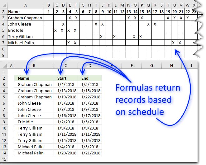
This article demonstrates ways to extract names and corresponding populated date ranges from a schedule using Excel 365 and earlier […]

Vlookup category

How to use VLOOKUP/XLOOKUP with multiple conditions
I will in this article demonstrate how to use the VLOOKUP function with multiple conditions. The function was not built […]

Excel categories

Comments (2)